Statforbiology
About this site
About me
Posts
Teaching material
Companion R Packages
Useful links
Fixing the bridge between biologists and statisticians
Categories
All
(13)
descriptive statistics
(2)
general
(1)
linear models
(1)
Mixed models
(1)
news
(2)
nlme
(1)
nonlinear regression
(4)
quarto
(1)
R
(9)
R-bloggers
(9)
Finally migrating to Quarto
An introduction with R
news
A few months ago, my
blogdown
-based blogs started giving me a few headaches, after more than seven years of remarkably reliable service. After doing some research on the web…
Jul 20, 2026
Andrea Onofri
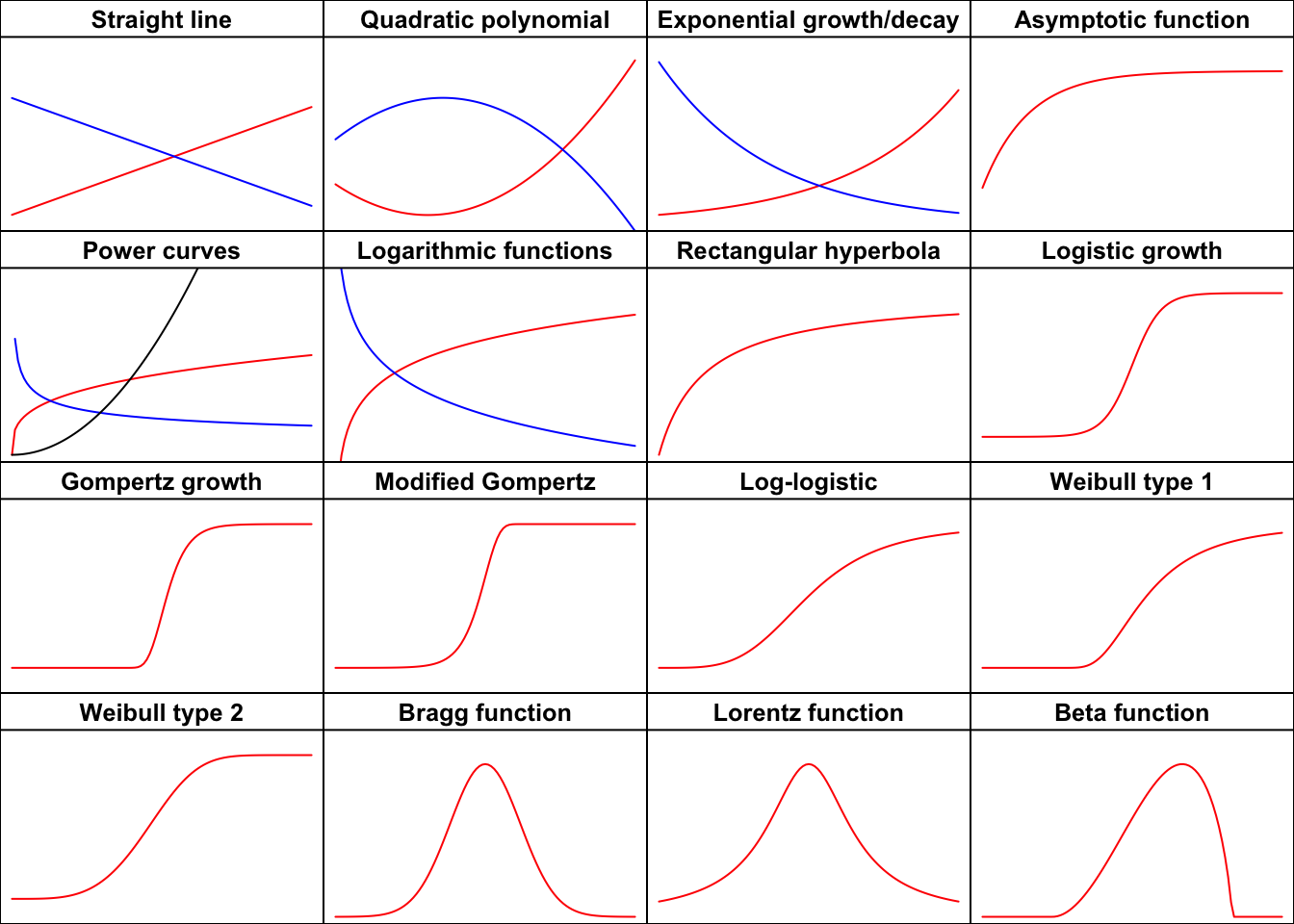
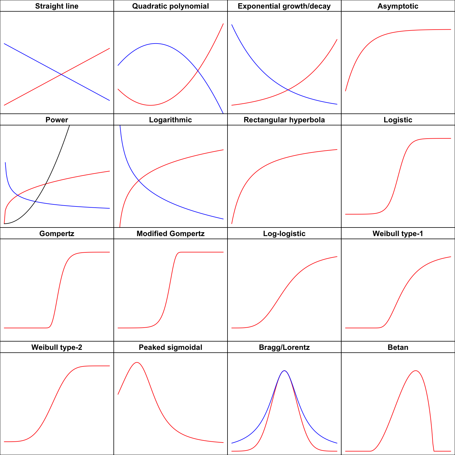
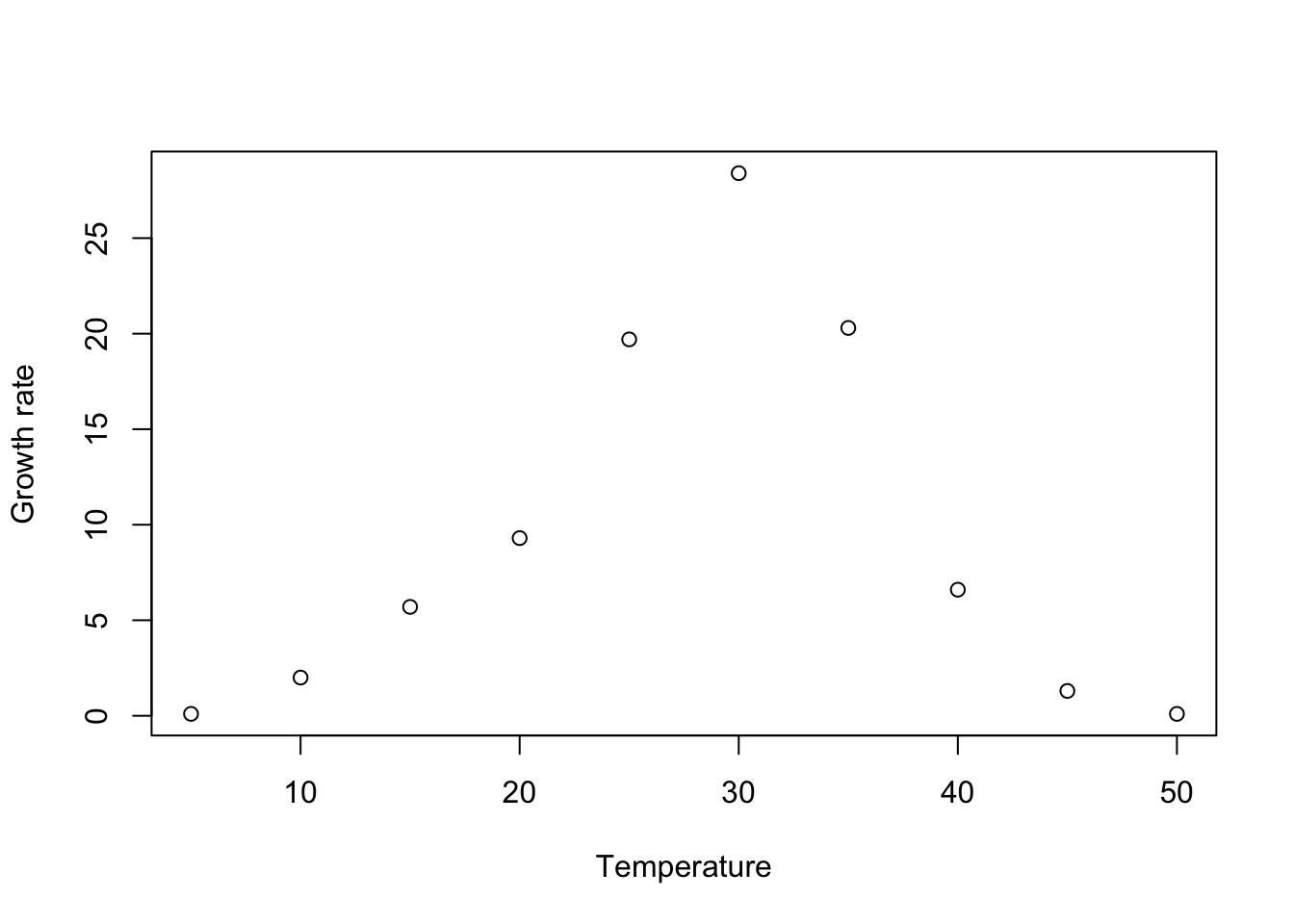
Some useful equations for biological processes
nonlinear regression
R-bloggers
Biological phenomena are often studied by examining how a numerical variable, usually called the
response
(e.g., the weight or height of an organism), is affected by another…
Jul 24, 2026
Andrea Onofri
A collection of self-starters for nonlinear regression in R
R
nonlinear regression
R-bloggers
Usually, the first step in every nonlinear regression analysis is to select the function
\(f\)
that best describes the phenomenon under study. The next step is to fit this…
Jul 21, 2026
Andrea Onofri
Migration from Blogdown to Quarto
R
quarto
More than twenty-five years ago, I had the idea that having a website would be a good way to store my teaching and research materials, keep them organised, retrieve them…
Jul 15, 2026
Andrea Onofri
How do we combine errors, in biology? The delta method
R
general
R-bloggers
In a recent post I have shown that we can build linear combinations of model parameters (see here ). For example, if we have two parameter estimates, say
\(X\)
and
\(Z\)
…
Dec 12, 2025
Andrea Onofri
Field Research methods in Agriculture
An introduction with R
news
Hi everybody, I have exciting news!
Nov 25, 2025
Andrea Onofri
How do we combine errors? The linear case
R
linear models
R-bloggers
In our research work, we usually fit models to experimental data. Our aim is to estimate some biologically relevant parameters, together with their standard errors. Very…
Nov 22, 2024
Andrea Onofri
Accounting for the experimental design in linear/nonlinear regression analyses
R
Mixed models
nonlinear regression
nlme
R-bloggers
In this post, I am going to talk about an issue that is often overlooked by agronomists and biologists. The point is that field experiments are very often laid down in…
Dec 4, 2020
Andrea Onofri
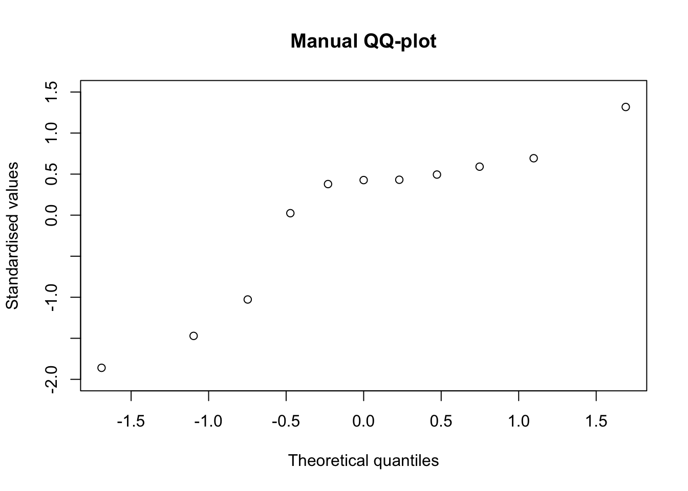
QQ-plots and Box-Whisker plots: where do they come from?
R
descriptive statistics
R-bloggers
This post is ‘only’ for the most curious students…
Oct 15, 2020
Andrea Onofri
Self-starting routines for nonlinear regression models
R
nonlinear regression
R-bloggers
In R, the
drc
package represents one of the main solutions for nonlinear regression and dose-response analyses (Ritz et al., 2015). It comes with a lot of nonlinear models…
Feb 14, 2020
Andrea Onofri
My learning path with blogdown
R
This is my first day at work with blogdown. I must admit it is pretty overwhelming at the beginning …
Nov 15, 2018
Andrea Onofri
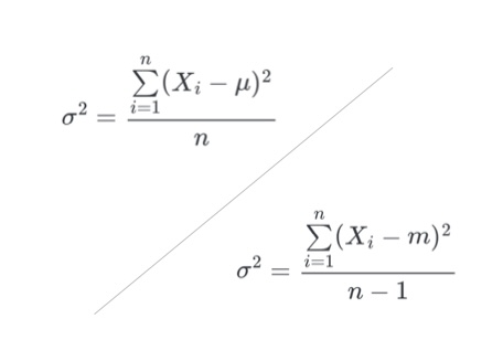
The Variance Puzzle: Why Doesn’t R Divide by ‘n’?
descriptive statistics
R-bloggers
Teaching Experimental Methodology in master’s courses related to agriculture poses some peculiar challenges. One of them is explaining the difference between
population…
Nov 9, 2018
Andrea Onofri
Is R dangerous? Side effects of free software for biologists
R
R-bloggers
When I started my career in biology (almost forty years ago), only the luckiest of us had access to advanced statistical software. Licences were very expensive, and it was…
Jun 8, 2014
Andrea Onofri
No matching items