During my stat courses, I never give my students any information about the Levene’s test (Levene and Howard, 1960), or other similar tests for homoscedasticity, unless I am specifically prompted to do so. It is not that I intend to underrate the tremendous importance of checking for the basic assumptions of linear model! On the contrary, I always show my students several methods for the graphical inspection of model residuals, but I do not share the same aching desire for a P-value, that most of my colleagues seem to possess.

I understand that the Levene’s test could have played an important role at the time when it was devised; at that time, biologists/agronomists used to only have ANOVA and regression at their disposal and the Levene’s or other formal tests were strictly necessary to assess whether those powerful techniques (ANOVA/regression) could be reliably used, in place of other less powerful non-parametric methods of data analyses. At that time, the only sensible question they could ask the data was: ‘are the variances homogeneous across the experimental groups?’. And the P-level from a Levene’s test provided the perfect answer.

Today, things have vastly changed: we have very powerful computers and we have the freeware statistical environment R, where an awful lot of advanced models are put at our disposal. There is nothing that prevents us from asking our body of data several interesting questions, such as:

1. do the treatments affect the variances of the experimental groups?
2. Are the variances, somehow, related to the expected responses?
3. Is a heteroscedastic model more reasonable than a homoscedastic model?

Nowadays, we can answer all these (and other) questions by an appropriate comparison of alternative models: for example, let’s consider a genotype experiment with kamut, resulting in the dataset ‘HetGenotypes.csv’, which is available in an external repository. It is a simple fully randomised experiment with three replicates, aimed at comparing the yield of 15 kamut genotypes.

library(dplyr)
fileName <- "https://www.casaonofri.it/_datasets/HetGenotypes.csv"
dataset <- read.csv(fileName)
dataset <- dataset |>
  transform(Genotype, factor(Genotype))
head(dataset)
##   Genotype Yield
## 1        A 8.129
## 2        A 8.616
## 3        A 7.932
## 4        B 6.188
## 5        B 6.767
## 6        B 6.635

It would be rather common to start the analyses by fitting a simple ‘ANOVA’ model, where the yield measurements (\(y_i\)) are regarded as functions of the ovarell mean (\(\mu\)) plus the genotype effects (\(\alpha_j\)), while errors (\(\varepsilon_i\)) are regarded as gaussian, independent and homoscedastic (a simple ANOVA model, indeed):

\[y_i = \mu + \alpha_j + \varepsilon_i; \quad \quad \textrm{with:} \quad \quad\varepsilon_i \sim N(0, \sigma)\]

For reasons that will be clearer later on, we fit this model by using the gls() function in the nlme package (same syntax as with the usual lm() function). Immediately afterwards, we plot the residuals, which reveals that there are strong differences of variability across groups, but residuals are not clearly related to yield level.

library(nlme)
library(ggplot2)
mod.aov <- gls(Yield ~ Genotype, data = dataset)

g1 <- ggplot(dataset) +
  geom_boxplot(mapping = aes(y = residuals(mod.aov), x = Genotype)) +
  theme_bw()
g2 <- ggplot() +
  geom_point(mapping = aes(y = residuals(mod.aov), x = fitted(mod.aov))) +
  theme_bw()
library(gridExtra)
gridExtra::grid.arrange(g1, g2, nrow = 1)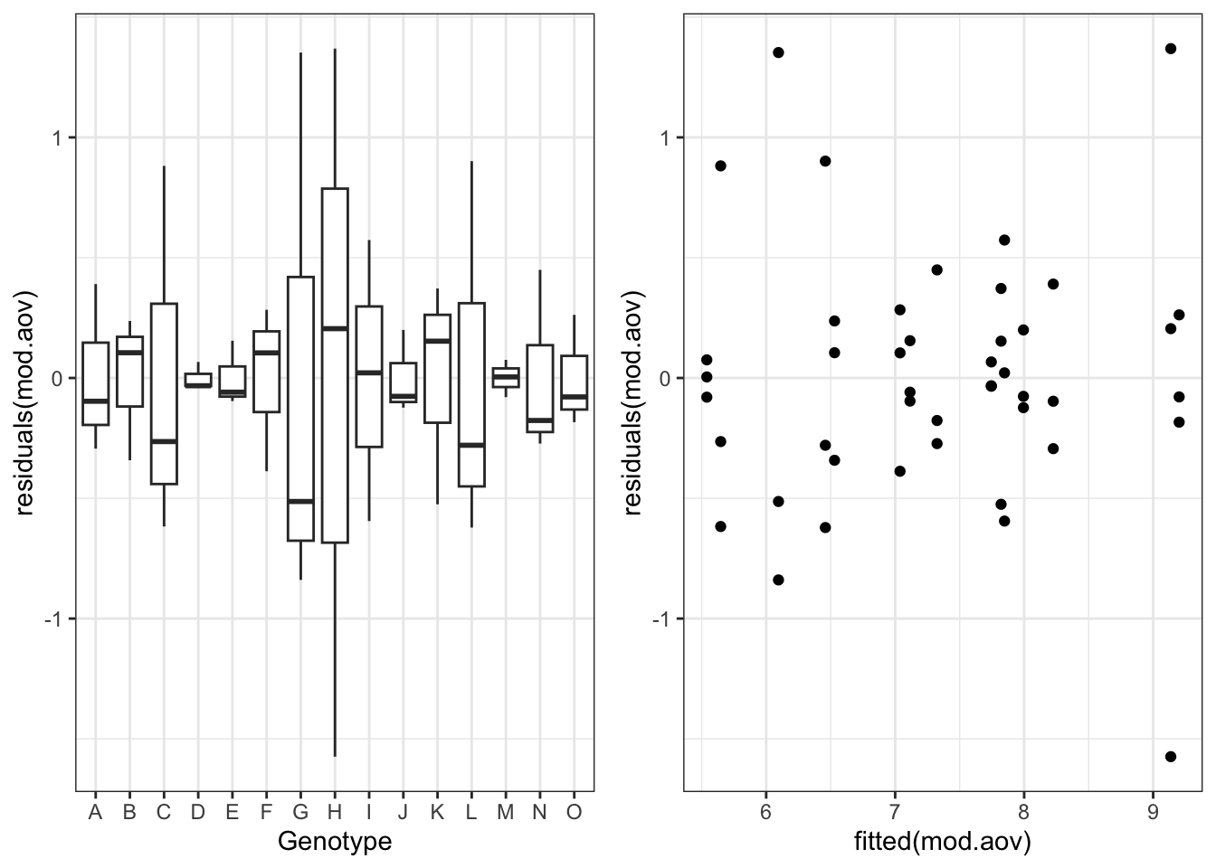 

My question at this stage: is it sensible to ask whether the variances are the same across groups? Using Tukey’s word (Tukey, 1991), such a question appears to be ‘rather foolish’, as the answer is already clear from the previous figure. However, it is sensible to ask whether a more complex model, allowing for heteroscedastic of within group errors, is warranted. Such a model would be expressed as:

\[y_i = \mu + \alpha_j + \varepsilon_i; \quad \quad \textrm{with:} \quad \quad\varepsilon_i \sim N(0, \sigma_j)\]

where \(\sigma_i\) is allowed to assume a different value for each genotype; nowadays, fitting such a model is widely feasible, by using the same gls() function as we have used before:

mod.het <- gls(Yield ~ Genotype, data = dataset,
               weights = varIdent(form = ~1|Genotype))

You see it: no fitting difficulties of any kind. This second model, with respect to the first one, may be more respectful of what we observed in our experiment, but it has the cost of requiring 14 extra parameters, to estimate 15 variances, instead of just one. Is this extra-cost justified by the data at hand?

We can directly compare the two models by using the AIC (Akaike’s information criterion):

anova(mod.aov, mod.het)
##         Model df       AIC      BIC    logLik   Test  L.Ratio p-value
## mod.aov     1 16 106.18435 128.6035 -37.09218                        
## mod.het     2 30  97.44571 139.4816 -18.72285 1 vs 2 36.73865   8e-04

We see that the AIC is lower for the heteroscedastic model and we also see that the Likelihood Ratio Test confirms that the more complex model is much more likely, in spite of the cost induced by the need for extra parameters. Thus I keep the most complex model and go ahead with that.

In conclusion, this is why I do not care about the Levene’s test: it provides a good answer to the wrong question (BTW: the Levene’s test in this circumstance turns out to be non-significant…)!

Thanks for reading and happy coding!

Andrea Onofri
Department of Agricultural, Food and Environmental Sciences
University of Perugia (Italy)
andrea.onofri@unipg.it

References

- Akaike, H., 1974. A new look at the statistical model identification. IEEE Transactions on Automatic Control 19, 716–723. https://doi.org/doi:10.1109/TAC.1974.1100705, MR 0423716
- Levene and Howard, 1960. Robust tests for equality of variances, In Ingram Olkin; Harold Hotelling; et al. (eds.), Contributions to Probability and Statistics: Essays in Honor of Harold Hotelling, Stanford University Press.
- Tukey, J.W., 1991. The phylosophy of multiple comparisons. Statistical Science 6, 100–116.