Again into a subject that is rather important for most agronomists, i.e. the selection of crop varieties. All farmers are perfectly aware that crop performances are affected both by the genotype and by the environment. These two effects are not purely additive and they often show a significant interaction. By this word, we mean that a genotype can give particularly good/bad performances in some specific environmental situations, which we may not expect, considering its average behaviour in other environmental conditions. The Genotype by Environment (GE) interaction may cause changes in the ranking of genotypes, depending on the environment and may play a key role in varietal recommendation, for a given mega-environment.
GE interactions are usually studied by way of Multi-Environment Trials (MET), where experiments are repeated across several years, locations or any combinations of those. Traditional techniques of data analyses, such as two-way ANOVA, give very little insight on the stability/reliability of genotypes across environments and, thus, other specialised techniques are necessary, to shed light on interaction effects. I have already talked about stability analyses in other posts, such as in this post about the stability variance or in this other post about the environmental variance. Now, I would like to propose some simple explanation about the AMMI analysis. AMMI stands for: Additive Main effect Multiplicative Interaction and it has become very much in fashion in the last 20-25 years.
Let’s start with a real MET example.
A MET with faba bean
This experiment consists of 12 faba bean genotypes (well, it was, indeed, 6 genotypes in two sowing dates; but, let’s disregard this detail from now on) in four blocks, two locations and three years (six environments, in all). The dataset is online available as ‘fabaBean.csv’ and it has been published by Stagnari et al. (2007).
First of all, let’s load the dataset and transform the block variable into a factor. Let’s also inspect the two-way table of means, together with the marginal means for genotypes and environments, which will be useful later. In this post, we will make use of the packages ‘dplyr’ (Wickham et al., 2020), ‘emmeans’ (Lenth, 2020) and ‘aomisc’; this latter is the companion package for this website and must have been installed as detailed in this page here.
# options(width = 70)

rm(list=ls())
# library(devtools)
# install_github("OnofriAndreaPG/aomisc")
library(reshape)
library(emmeans)
library(aomisc)

fileName <- "https://www.casaonofri.it/_datasets/fabaBean.csv"
dataset <- read.csv(fileName, header=T)
dataset <- transform(dataset, Block = factor(Block),
                     Genotype = factor(Genotype),
                     Environment = factor(Environment))
head(dataset)
##      Genotype Block Environment Yield
## 1    Chiaro_A     1       bad_1  4.36
## 2    Chiaro_P     1       bad_1  2.76
## 3 Collameno_A     1       bad_1  3.01
## 4 Collameno_P     1       bad_1  2.50
## 5    Palomb_A     1       bad_1  3.85
## 6    Palomb_P     1       bad_1  2.21
#
# Two-ways table of means
GEmedie <- cast(Genotype ~ Environment, data = dataset,
                value = "Yield", fun=mean)
GEmedie
##       Genotype  bad_1  bad_2  bad_3  pap_1  pap_2  pap_3
## 1     Chiaro_A 4.1050 2.3400 4.1250 4.6325 2.4100 3.8500
## 2     Chiaro_P 2.5075 1.3325 4.2025 3.3225 1.4050 4.3175
## 3  Collameno_A 3.2500 2.1150 4.3825 3.8475 2.2325 4.0700
## 4  Collameno_P 1.9075 0.8475 3.8650 2.5200 0.9850 4.0525
## 5     Palomb_A 3.8400 2.0750 4.2050 5.0525 2.6850 4.6675
## 6     Palomb_P 2.2500 0.9725 3.2575 3.2700 0.8825 4.0125
## 7      Scuro_A 4.3700 2.1050 4.1525 4.8625 2.1275 4.2050
## 8      Scuro_P 3.0500 1.6375 3.9300 3.7200 1.7475 4.5125
## 9    Sicania_A 3.8300 1.9450 4.5050 3.9550 2.2350 4.2350
## 10   Sicania_P 3.2700 0.9900 3.7300 4.0475 0.8225 3.8950
## 11   Vesuvio_A 4.1375 2.0175 4.0275 4.5025 2.2650 4.3225
## 12   Vesuvio_P 2.1225 1.1800 3.5250 3.0950 0.9375 3.6275
#
# Marginal means for genotypes
apply(GEmedie, 1, mean)
##    Chiaro_A    Chiaro_P Collameno_A Collameno_P    Palomb_A
##    3.577083    2.847917    3.316250    2.362917    3.754167
##    Palomb_P     Scuro_A     Scuro_P   Sicania_A   Sicania_P
##    2.440833    3.637083    3.099583    3.450833    2.792500
##   Vesuvio_A   Vesuvio_P
##    3.545417    2.414583
#
# Marginal means for environments
apply(GEmedie, 2, mean)
##    bad_1    bad_2    bad_3    pap_1    pap_2    pap_3
## 3.220000 1.629792 3.992292 3.902292 1.727917 4.147292
#
# Overall mean
mean(as.matrix(GEmedie))
## [1] 3.103264
What model could we possibly fit to the above data? The basic two-way ANOVA model is:
\[Y_{ijk} = \mu + \gamma_{jk} + g_i + e_j + ge_{ij} + \varepsilon_{ijk} \quad \quad (1)\]
where the yield \(Y\) for given block \(k\), environment \(j\) and genotype \(i\) is described as a function of the effects of blocks within environments (\(\gamma\)), genotypes (\(g\)), environments (\(e\)) and GE interaction (\(ge\)). The residual error term \(\varepsilon\) is assumed to be normal and homoscedastic, with standard deviation equal to \(\sigma\). Let’s also assume that both the genotype and environment effects are fixed: this is useful for teaching purposes and it is reasonable, as we intend to study the behaviour of specific genotypes in several specific environments.
The interaction effects (and GE matrix)
The interaction effect \(ge\), under some important assumptions (i.e. balanced data, no missing cells and homoscedastic errors), is given by:
\[ge_{ij} = Y_{ij.} - \left( \mu + g_i + e_j \right) = Y_{ij.} - Y_{i..} - Y_{.j.} + \mu \quad \quad (2)\]
where \(Y_{ij.}\) is the mean of the combination between the genotype \(i\) and the environment \(j\), \(Y_{i..}\) is the mean for the genotype \(i\) and \(Y_{.j.}\) is the mean for the environment \(j\). For example, for the genotype ‘Chiaro_A’ in the environment ‘bad_1’, the interaction effect was:
4.1050 - 3.577 - 3.22 + 3.103
## [1] 0.411
We see that the interaction was positive, in the sense that ‘Chiaro_A’, gave 0.411 tons per hectare more than we could have expected, considering its average performances across environments and the average performances of all genotypes in ‘bad_1’.
It may be very handy to organise the interaction effects in a two-way table, with the genotypes along the rows and environments along the columns (or vice-versa, as you prefer). Such a two-way table can be simply obtained by doubly centring the matrix of means, as shown in the following box.
GE <- as.data.frame(t(scale( t(scale(GEmedie, center=T,
 scale=F)), center=T, scale=F)))
print(round(GE, 3))
##              bad_1  bad_2  bad_3  pap_1  pap_2  pap_3
## Chiaro_A     0.411  0.236 -0.341  0.256  0.208 -0.771
## Chiaro_P    -0.457 -0.042  0.466 -0.324 -0.068  0.426
## Collameno_A -0.183  0.272  0.177 -0.268  0.292 -0.290
## Collameno_P -0.572 -0.042  0.613 -0.642 -0.003  0.646
## Palomb_A    -0.031 -0.206 -0.438  0.499  0.306 -0.131
## Palomb_P    -0.308  0.005 -0.072  0.030 -0.183  0.528
## Scuro_A      0.616 -0.059 -0.374  0.426 -0.134 -0.476
## Scuro_P     -0.166  0.011 -0.059 -0.179  0.023  0.369
## Sicania_A    0.262 -0.032  0.165 -0.295  0.160 -0.260
## Sicania_P    0.361 -0.329  0.048  0.456 -0.595  0.058
## Vesuvio_A    0.475 -0.054 -0.407  0.158  0.095 -0.267
## Vesuvio_P   -0.409  0.239  0.221 -0.119 -0.102  0.169
Please, note that the overall mean for all elements in ‘GE’ is zero and the sum of squares is equal to a fraction of the interaction sum of squares in ANOVA (that is \(RMSE/r\); where \(r\) is the number of blocks).
mean(unlist(GE))
## [1] 6.914424e-18
sum(GE^2)
## [1] 7.742996
mod <- lm(Yield ~ Environment/Block + Genotype*Environment, data = dataset)
anova(mod)
## Analysis of Variance Table
##
## Response: Yield
##                       Df Sum Sq Mean Sq  F value    Pr(>F)
## Environment            5 316.57  63.313 580.9181 < 2.2e-16 ***
## Genotype              11  70.03   6.366  58.4111 < 2.2e-16 ***
## Environment:Block     18   6.76   0.375   3.4450 8.724e-06 ***
## Environment:Genotype  55  30.97   0.563   5.1669 < 2.2e-16 ***
## Residuals            198  21.58   0.109
## ---
## Signif. codes:  0 '***' 0.001 '**' 0.01 '*' 0.05 '.' 0.1 ' ' 1
30.97/4
## [1] 7.7425
Decomposing the GE matrix
It would be nice to be able to give a graphical summary of the GE matrix; in this regard, we could think of using Principal Component Analysis (PCA) via Singular Value Decomposition (SVD). This has been shown by Zobel et al. (1988) and, formerly, by Gollob (1968). May I just remind you a few things about PCA and SVD? No overwhelming math detail, I promise!
Most matrices (and our GE matrix) can be decomposed as the product of three matrices, according to:
\[X = U D V^T \quad \quad (3)\]
where \(X\) is the matrix to be decomposed, \(U\) is the matrix of the first \(n\) eigenvectors of \(XX^T\), \(V\) is the matrix of the first \(n\) eigenvectors of \(X^T X\) and \(D\) is the diagonal matrix of the first \(n\) singular values of \(XX^T\) (or \(X^T X\); it does not matter, they are the same).
Indeed, if we want to decompose our GE matrix, it is more clever (and more useful to our purposes), to write the following matrices:
\[S_g = U D^{1/2} \quad \quad (4)\]
and:
\[S_e = V D^{1/2} \quad \quad (5)\]
so that
\[GE = S_g \, S_e^T \quad \quad (6)\]
\(S_g\) is the matrix of row-scores (genotype scores) and \(S_e\) is the matrix of column scores (environment scores). Let me give you an empirical proof, in the box below. In order to find \(S_g\) and \(S_e\), I will use a mathematical operation that is known as Singular Value Decomposition (SVD):
U <- svd(GE)$u
V <- svd(GE)$v
D <- diag(svd(GE)$d)
Sg <- U %*% sqrt(D)
Se <- V %*% sqrt(D)
row.names(Sg) <- levels(dataset$Genotype)
row.names(Se) <- levels(dataset$Environment)
colnames(Sg) <- colnames(Se) <- paste("PC", 1:6, sep ="")
round(Sg %*% t(Se), 3)
##              bad_1  bad_2  bad_3  pap_1  pap_2  pap_3
## Chiaro_A     0.411  0.236 -0.341  0.256  0.208 -0.771
## Chiaro_P    -0.457 -0.042  0.466 -0.324 -0.068  0.426
## Collameno_A -0.183  0.272  0.177 -0.268  0.292 -0.290
## Collameno_P -0.572 -0.042  0.613 -0.642 -0.003  0.646
## Palomb_A    -0.031 -0.206 -0.438  0.499  0.306 -0.131
## Palomb_P    -0.308  0.005 -0.072  0.030 -0.183  0.528
## Scuro_A      0.616 -0.059 -0.374  0.426 -0.134 -0.476
## Scuro_P     -0.166  0.011 -0.059 -0.179  0.023  0.369
## Sicania_A    0.262 -0.032  0.165 -0.295  0.160 -0.260
## Sicania_P    0.361 -0.329  0.048  0.456 -0.595  0.058
## Vesuvio_A    0.475 -0.054 -0.407  0.158  0.095 -0.267
## Vesuvio_P   -0.409  0.239  0.221 -0.119 -0.102  0.169
Let’s have a look at \(S_g\) and \(S_e\): they are two interesting entities. I will round up a little to make them smaller, and less scaring.
round(Sg, 3)
##                PC1    PC2    PC3    PC4    PC5 PC6
## Chiaro_A    -0.607 -0.384  0.001  0.208 -0.063   0
## Chiaro_P     0.552  0.027 -0.081  0.045  0.164   0
## Collameno_A  0.084 -0.542 -0.006  0.176  0.057   0
## Collameno_P  0.807 -0.066 -0.132 -0.172  0.079   0
## Palomb_A    -0.321  0.110  0.591 -0.083  0.389   0
## Palomb_P     0.281  0.346  0.282  0.042 -0.253   0
## Scuro_A     -0.626  0.139 -0.163  0.017 -0.080   0
## Scuro_P      0.230  0.077  0.182 -0.207 -0.242   0
## Sicania_A   -0.063 -0.324 -0.355 -0.280  0.090   0
## Sicania_P   -0.214  0.683 -0.402  0.148  0.151   0
## Vesuvio_A   -0.438 -0.008  0.020 -0.300 -0.177   0
## Vesuvio_P    0.316 -0.058  0.063  0.405 -0.114   0
round(Se, 3)
##          PC1    PC2    PC3    PC4    PC5 PC6
## bad_1 -0.831  0.095 -0.467 -0.317 -0.151   0
## bad_2  0.044 -0.418  0.070  0.371 -0.403   0
## bad_3  0.670 -0.130 -0.525  0.171  0.298   0
## pap_1 -0.661  0.513  0.289  0.314  0.221   0
## pap_2 -0.069 -0.627  0.420 -0.294  0.208   0
## pap_3  0.846  0.567  0.213 -0.244 -0.173   0
Both matrices have 6 columns. Why six, are you asking? I promised I would not go into math detail; it’s enough to know that the number of columns is always equal to the minimum value between the number of genotypes and the number of environments. The final column is irrelevant (all elements are 0). \(S_g\) has 12 rows, one per genotype; these are the so called genotype scores: each genotype has six scores. \(S_e\) has six rows, one per environment (environment scores).
You may have some ‘rusty’ memories about matrix multiplication; however, what we have discovered in the code box above is that the GE interaction for the \(i^{th}\) genotype and the \(j^{th}\) environment can be obtained as the product of genotype scores and environments scores. Indeed:
\[ge_{ij} = \sum_{z = 1}^n \left[ S_g(iz) \cdot S_e(jz) \right] \quad \quad (7)\]
where \(n\) is the number of columns (number of principal components). An example is in order, at this point; again, let’s consider the first genotype and the first environment. The genotype and environments scores are in the first columns of \(S_g\) and \(S_e\); if we multiply the elements in the same positioning (1st with 1st, 2nd with 2nd, and so on) and sum up, we get:
-0.607 * -0.831 +
-0.384 *  0.095 +
 0.001 * -0.467 +
 0.208 * -0.317 +
-0.063 * -0.151 +
     0 * 0
## [1] 0.411047
It’s done: we have transformed the interaction effect into the sum of multiplicative terms. If we replace Equation 7 into the ANOVA model above (Equation 1), we obtain an Additive Main effects Multiplicative Interaction model, i.e. an AMMI model.
Reducing the rank
In this case we took all available columns in \(S_g\) and \(S_e\). For the sake of simplicity, we could have taken only a subset of those columns. The Eckart-Young (1936) theorem says that, if we take \(m < 6\) columns, we obtain the best possible approximation of GE in reduced rank space. For example, let’s use the first two columns of \(S_g\) and \(S_e\) (the first two principal component scores):
PC <- 2
Sg2 <- Sg[,1:PC]
Se2 <- Se[,1:PC]
GE2 <- Sg2 %*% t(Se2)
print ( round(GE2, 3) )
##              bad_1  bad_2  bad_3  pap_1  pap_2  pap_3
## Chiaro_A     0.468  0.134 -0.357  0.205  0.282 -0.732
## Chiaro_P    -0.456  0.013  0.367 -0.351 -0.055  0.482
## Collameno_A -0.122  0.230  0.127 -0.334  0.334 -0.236
## Collameno_P -0.676  0.063  0.549 -0.567 -0.014  0.645
## Palomb_A     0.277 -0.060 -0.230  0.269 -0.047 -0.209
## Palomb_P    -0.201 -0.132  0.144 -0.009 -0.236  0.434
## Scuro_A      0.534 -0.086 -0.438  0.486 -0.044 -0.451
## Scuro_P     -0.184 -0.022  0.144 -0.113 -0.064  0.238
## Sicania_A    0.022  0.133  0.000 -0.124  0.207 -0.237
## Sicania_P    0.243 -0.295 -0.232  0.492 -0.414  0.206
## Vesuvio_A    0.363 -0.016 -0.293  0.286  0.035 -0.375
## Vesuvio_P   -0.268  0.038  0.219 -0.239  0.015  0.234
GE2 is not equal to GE, but it is a close approximation. A close approximation in what sense?… you may wonder. Well, the sum of squared elements in GE2 is as close as possible (with \(n = 2\)) to the sum of squared elements in GE:
sum(GE2^2)
## [1] 6.678985
We see that the sum of squares in GE2 is 86% of the sum of squares in GE. A very good approximation, isn’t it? It means that the variability of yield across environments is described well enough by using a relatively low number of parameters (scores). However, the multiplicative part of our AMMI model needs to be modified:
\[ge_{ij} = \sum_{z = 1}^m \left[ s_{g(iz)} \cdot s_{e(jz)} \right] + \xi_{ij}\]
Indeed, a residual term \(\xi_{ij}\) is necessary, to account for the fact that the sum of multiplicative terms is not able to fully recover the original matrix GE. Another example? For the first genotype and the first environment the multiplicative interaction is:
-0.607 * -0.831 + -0.384 * 0.095
## [1] 0.467937
and the residual term \(\xi_{11}\) is
0.41118056 -0.607 * -0.831 + -0.384 * 0.095
## [1] 0.8791176
Clearly, the residual terms need to be small enough to be negligible, otherwise the approximation in reduced rank space is not good enough.
Why is this useful?
Did you get lost? Hope you didn’t, but let’s make a stop and see where we are standing now. We started from the interaction matrix GE and found a way to decompose it as the product of two matrices, i.e. \(S_g\) and \(S_e\), a matrix of genotype scores and a matrix of environment scores. We discovered that we could obtain a good approximation of GE by working in reduced rank space and we only used two genotypic scores and two environment scores, in place of the available six.
This is great! Now we have the ability of drawing a biplot, i.e. we can plot both genotypic scores and environmental scores in a dispersion graph (biplot: two plots in one), as we see below.
biplot(Sg[,1:2], Se[,1:2], xlim = c(-1, 1), ylim = c(-1, 1),
       xlab = "PC 1", ylab = "PC 2")
abline(h = 0, lty = 2)
abline(v = 0, lty = 2)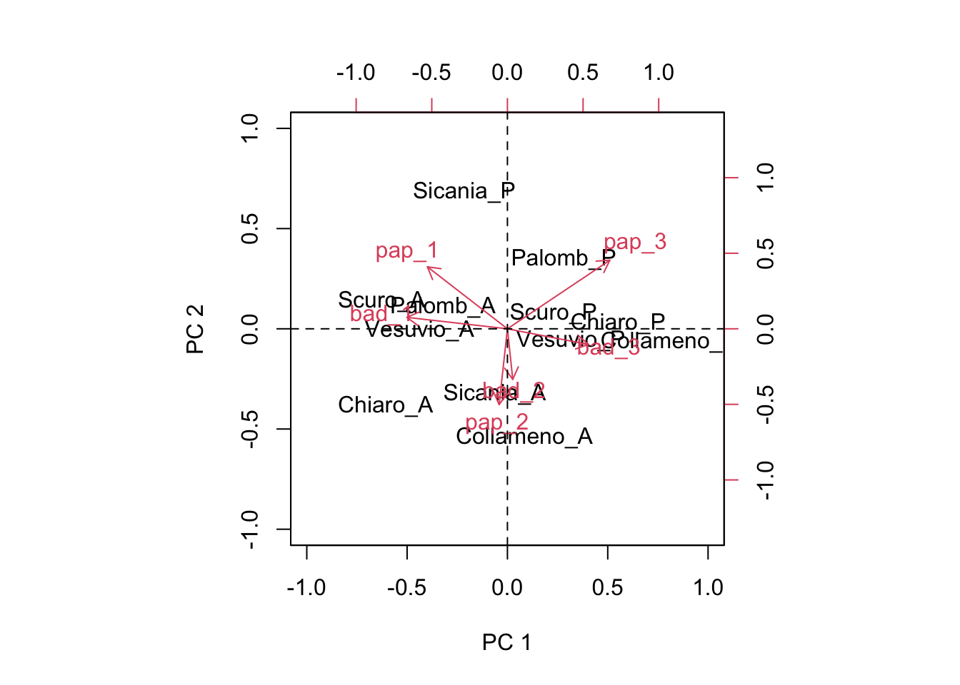
This graph provides a very effective description of GE interaction effects. I will not go into detail, here. Just a few simple comments:
- genotypes and environments lying close to the origin of the axes do not interact with each other (the product of scores would be close to 0)
- genotypes and environments lying far away from the origin of axes show very big interaction and, therefore, high yield instability. Someone says that the euclidean distance from the origin should be taken as a measure of instability
- the interaction is positive, when genotypes and environments are close to each other. If two objects are close, their scores (co-ordinates) will have the same signs and thus their product will be positive.
- the interaction is negative, when genotypes and environments are far away from each other. If two objects are distant, their scores (co-ordinates) will have opposte signs and thus their product will be negative.
- For instance, ‘Palomb_P’, ‘Scuro_P’, ‘Chiaro_P’ and ‘Collameno_P’ gave particularly good yields in the environments ‘pap_3’ and ‘bad_3’, while ‘Scuro_A’, ‘Palomb_A’ and ‘Vesuvio_A’ gave particularly good yields (compared to their average) in the environments ‘pap_1’ and ‘bad_1’. ‘Sicania_A’ and ‘Collameno_A’ gave good yields in ‘bad_2’ and ‘pap_2’.
How many components?
In my opinion, AMMI analysis is mainly a visualisation method. Therefore, we should select as many components (columns in \(S_g\) and \(S_e\)) as necessary to describe a main part of the interaction sum of squares. In our example, two components are enough, as they represent 86% of the interaction sum of squares.
However, many people (and reviewers) are still very concerned with formal hypothesis testing. Therefore, we could proceed in a sequential fashion, and introduce the components one by one.
The first component has a sum of squares equal to:
PC <- 1
Sg2 <- Sg[,1:PC]
Se2 <- Se[,1:PC]
GE2 <- Sg2 %*% t(Se2)
sum(GE2^2)
## [1] 5.290174
We have seen that the second component has an additional sum of squares equal to:
6.678985 - 5.290174
## [1] 1.388811
We can go further ahead and get the sum of squares for all components. According to Zobel (1988), the degrees of freedom for each component are equal to:
\[ df_n = i + j - 1 - 2m \]
where \(i\) is the number of genotypes, \(j\) is the number of environments, and \(m\) is the number of the selected components. In our case, the first PC has 15 DF, the second one has 13 DF and so on.
If we can have a reliable estimate of the pure error variance \(\sigma^2\) (see above), we can test the significance of each component by using F tests (although some authors argue that this is too a liberal approach; see Cornelius, 1993).
Simple AMMI analysis with R
We have seen that AMMI analysis, under the hood, is a sort of PCA. Therefore, it could be performed, in R by using one of the available packages for PCA. For the sake of simplicity, I have coded the simple AMMI() function, that is available in the ‘aomisc’ package. I have described an earlier version of this function in an ‘R news’ paper (Onofri and Ciriciofolo, 2007).
Tha above function works equally well with raw MET data, containing all replicated values, or with the ‘genotype by environment’ average values. In this second case, the analyses proceed in two-steps, as I will describe below.
First step on raw data
During the first step we need to obtain a reliable matrix of means for the ‘genotype x environment’ combinations. If the environment is fixed, we can use least squares means, which are unbiased, also when some observations are missing. If the environment effect is random, we could use the BLUPs, but we will not consider such an option here.
In the box below we take the ‘mod’ object from a two way ANOVA fit and derive the residual mean square (RMSE), which we divide by the number of blocks. This will be our error term to test the significance of components. Later, we pass the ‘mod’ object to the ‘emmeans()’ function, to retrieve the expected marginal means for the ‘genotype by environment’ combinations and proceed to the second step.
RMSE <- summary(mod)$sigma^2 / 4
dfr <- mod$df.residual
ge.lsm <- emmeans(mod, ~Genotype:Environment)
ge.lsm <- data.frame(ge.lsm)[,1:3]
Second step on least square means
This second step assumes that the residual variances for all environments are homogeneous. If so (we’d better check this), we can take the expected marginal means (‘ge.lsm’) and submit them to AMMI analysis, by using the AMMI() function. The syntax is fairly obvious; we also pass to it the RMSE and its degrees of freedom. The resulting object can be explored, by using the appropriate slots.
AMMIobj <- AMMI(yield = ge.lsm$emmean,
                     genotype = ge.lsm$Genotype,
                     environment = ge.lsm$Environment,
                     MSE = RMSE, dfr = dfr)
#
AMMIobj$genotype_scores
##                     PC1          PC2
## Chiaro_A    -0.60710888 -0.383732821
## Chiaro_P     0.55192742  0.026531045
## Collameno_A  0.08444877 -0.542185666
## Collameno_P  0.80677055 -0.065752971
## Palomb_A    -0.32130513  0.110117240
## Palomb_P     0.28104959  0.345909298
## Scuro_A     -0.62638795  0.139185954
## Scuro_P      0.22961347  0.076555540
## Sicania_A   -0.06286803 -0.323857285
## Sicania_P   -0.21433211  0.683296898
## Vesuvio_A   -0.43786742 -0.007914342
## Vesuvio_P    0.31605973 -0.058152890
#
AMMIobj$environment_scores
##               PC1         PC2
## bad_1 -0.83078550  0.09477362
## bad_2  0.04401963 -0.41801637
## bad_3  0.67043214 -0.12977423
## pap_1 -0.66137357  0.51268429
## pap_2 -0.06863235 -0.62703224
## pap_3  0.84633965  0.56736492
#
AMMIobj$mult_Interaction
##      Effect       SS DF        MS         F        Prob. Perc_of_Total_SS
## 1       PC1 5.290174 15 0.3526782 12.943700 2.926881e-22        0.6832205
## 2       PC2 1.388812 13 0.1068317  3.920847 1.135641e-05        0.1793636
## 3 Residuals 1.064011 27 0.0394078  1.446312 8.056050e-02        0.1374159
In detail, we can retrieve the genotype and environment scores, the proportion of the GE variance explained by each component and the significance of PCs.
I agree, the AMMI() function is not very ambitious. However, it is simple enough to be usable and give reliable results, as long as the basic assumptions for the method are respected. Furthermore, there is also a complimentary biplot() method, that draws either the biplot type 1 (PC1 for genotypes and environments against genotypic/environment means) or the biplot type 2 (PC1 against PC2). The code is shown below.
biplot(AMMIobj, xlab = "Yield")
biplot(AMMIobj, biplot = 2)
You may also consider to explore other more comprehensive R packages, such as ‘agricolae’ (de Mendiburu, 2020).
Thank you for reading, so far, and… happy coding!
Prof. Andrea Onofri
Department of Agricultural, Food and Environmental Sciences
University of Perugia (Italy)
Send comments to: andrea.onofri@unipg.it
Literature references
- Annichiarico, P. (1997). Additive main effects and multiplicative interaction (AMMI) analysis of genotype-location interaction in variety trials repeated over years. Theoretical applied genetics, 94, 1072-1077.
- Ariyo, O. J. (1998). Use of additive main effects and multiplicative interaction model to analyse multilocation soybean varietal trials. J. Genet. and Breed, 129-134.
- Cornelius, P. L. (1993). Statistical tests and retention of terms in the Additive Main Effects and Multiplicative interaction model for cultivar trials. Crop Science, 33,1186-1193.
- Crossa, J. (1990). Statistical Analyses of multilocation trials. Advances in Agronomy, 44, 55-85.
- Gollob, H. F. (1968). A statistical model which combines features of factor analytic and analysis of variance techniques. Psychometrika, 33, 73-114.
- Lenth R., 2020. emmeans: Estimated Marginal Means, aka Least-Squares Means. R package version 1.4.6. https://github.com/rvlenth/emmeans.
- de Mendiburu F., 2020. agricolae: Statistical Procedures for Agricultural Research. R package version 1.3-2. https://CRAN.R-project.org/package=agricolae.
- Onofri, A., Ciriciofolo, E., 2007. Using R to perform the AMMI analysis on agriculture variety trials. R NEWS 7, 14–19.
- Stagnari F., Onofri A., Jemison J., Monotti M. (2006). Multivariate analyses to discriminate the behaviour of faba bean (Vicia faba L. var. minor) varieties as affected by sowing time in cool, low rainfall Mediterranean environments. Agronomy For Sustainable Development, 27, 387–397.
- Hadley Wickham, Romain François, Lionel Henry and Kirill Müller, 2020. dplyr: A Grammar of Data Manipulation. R package version 0.8.5. https://CRAN.R-project.org/package=dplyr.
- Zobel, R. W., Wright, M.J., and Gauch, H. G. (1988). Statistical analysis of a yield trial. Agronomy Journal, 388-393.