Fitting hydro-time-to-event models

Let’s consider the following example: the germination of rapeseed (Brassica napus L. var. oleifera, cv. Excalibur) was tested at fourteen different water potential levels (0, -0.03, -0.15, -0.3, -0.4, -0.5, -0.6, -0.7, -0.8, -0.9, -1, -1.1, -1.2, -1.5 MPa), which were created by using a polyethylene glycol solution (PEG 6000). For each water potential level, three replicated Petri dishes with 50 seeds each were incubated at 20°C. Germinated seeds were counted every 2-3 days for 14 days and they were removed from the dishes after germination.

The dataset was published by Pace et al. (2012) and it is available as rape in the drcSeedGerm package, which needs to be installed from github (see below). Furthermore, the package drcte is necessary to fit time-to-event models and it should also be installed from gitHub. The following code loads the necessary packages, loads the dataset rape and shows the first six lines.

# install.packages("drcte")
# install.packages("drcSeedGerm")
library(drcte)
library(drcSeedGerm)
library(ggplot2)
data(rape)
head(rape)
##   Psi Dish timeBef timeAf nSeeds nCum propCum
## 1   0    1       0      3     49   49    0.98
## 2   0    1       3      4      0   49    0.98
## 3   0    1       4      5      0   49    0.98
## 4   0    1       5      7      0   49    0.98
## 5   0    1       7     10      0   49    0.98
## 6   0    1      10     14      0   49    0.98

In the above data.frame, ‘timeAf’ represents the moment when germinated seeds were counted, while ’timeBef’ represents the previous inspection time (or the beginning of the assay). The column ’nSeeds’ is the number of seeds that germinated during the time interval between ‘timeBef’ and ’timeAf. The ’propCum’ column contains the cumulative proportions of germinated seeds and it is not necessary for time-to-event model fitting, although we can use it for plotting purposes (see code and output below).

ggplot(rape, aes(timeAf, propCum)) +
  geom_point() +
  facet_wrap(~Psi) +
  scale_x_continuous(name = "Time (d)") +
  scale_y_continuous(name = "Cumulative proportion of germinated seeds") +
  theme_bw()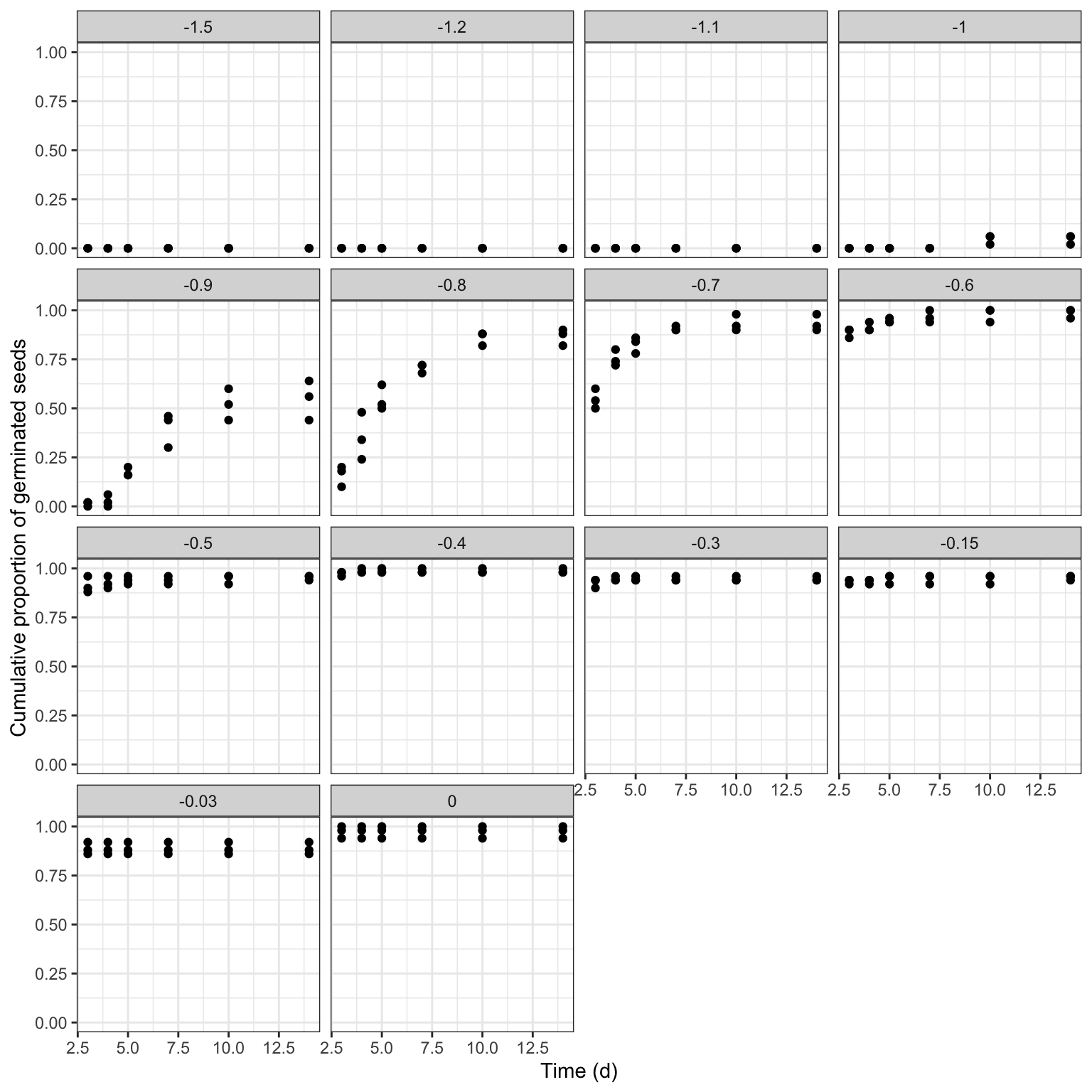

The germination time course is strongly influenced by substrate water potential, which regulates seed water uptake and thus the initiation of germination and emergence. Our goal is therefore to quantify how this environmental factor shapes germination dynamics over time.

We have shown that a parametric time-to-event curve is defined as a cumulative probability function (\(\Phi\)), with three parameters:

\[P(t) = \Phi \left( b, d, e \right)\] Let’s see how we can incorporate an environmental covariate in this curve.

Suboptimal approach

Considering our previous post, the most obvious extension of the above model is to allow for different \(b\), \(d\) and \(e\) value for each water potential level:

\[P(t, \Psi_i) = \Phi \left( b_i, d_i, e_i \right)\]

The first issue is that, at some water potential levels, germination did not occur at all, whereas at other levels it occurred so rapidly that no meaningful time course could be observed (e.g. see the graph at 0 or −0.03 MPa). We refer to these as degenerated time-to-event curves.

The presence of such degenerated curves prevents successful model fitting, as the curveid argument imposes a common time-to-event structure across all water potential levels, which is not appropriate in this case.

# Not run
# mod0 <- drmte(nSeeds ~ timeBef + timeAf, data = rape,
#              curveid = Psi, fct = loglogistic())

This problem can be circumvented by using the separate = TRUE argument; in this case, the different curves are fitted independent of one another and we are not tied to fitting the same model for all water potential levels.

mod1 <- drmte(nSeeds ~ timeBef + timeAf, data = rape,
             curveid = Psi, fct = loglogistic(),
             separate = TRUE)
coef(mod1)
 #    d:-1.5      d:-1.2      d:-1.1        b:-1        d:-1        e:-1      b:-0.9 
 # 0.00000000  0.00000000  0.00000000 64.39202307  0.04666194  8.36474946  5.83290900 
 #     d:-0.9      e:-0.9      b:-0.8      d:-0.8      e:-0.8      b:-0.7      d:-0.7 
 # 0.55010281  5.87022056  3.73294999  0.87889318  4.47105672  3.59940891  0.93592886 
 #     e:-0.7      b:-0.6      e:-0.6      b:-0.5      e:-0.5      d:-0.4      d:-0.3 
 # 2.73025095  1.46592984  0.73866435  0.59257691  0.05876917  0.98444444  0.94333333 
 #    b:-0.15     e:-0.15     d:-0.03         d:0 
 # 0.55872202  0.02997354  0.88666667  0.97333333 

In particular, for the cases where a time-course of events cannot be estimated, an error message is shown, but the execution of codes is not stopped and the drmte() function resorts to fitting a simpler model, where only the \(d\) parameter is estimated (that is the maximum fraction of germinated seeds). In the box above, we can see the estimated parameters but no standard errors, which can be obtained by using the summary() method, although there are some statistical issues that we will consider in a following post.

A better modelling approach

The previous approach is clearly sub-optimal. First of all, the different water potential levels are assumed as independent, with no ordering and distances. In other words, we have a time-to-event curve for, e.g. -0.9 MPa and -0.8 MPa, but we have no information about the time-to-event curve for any water potential levels in between. Furthermore, we have no estimates of some relevant hydro-time parameters, such as the base water potential, that is fundamental to predict the germination/emergence in field conditions.

In order to account for the very nature of the water potential variable, we could code a time-to-event model where the three parameters are continuous functions of \(\Psi\):

\[P(t, \Psi) = \Phi \left( b(\Psi), d(\Psi), e(\Psi) \right)\]

We followed such an approach in a relatively recent publication (Onofri et al., 2018) and we also spoke about this in a recent post. In detail, we considered a log-logistic cumulative distribution function:

\[P(t) = \frac{ d }{1 + \exp \left\{ b \left[ \log(t) - \log( e ) \right] \right\} }\]

where \(e\) is the median germination time, \(b\) is the slope at the inflection point and \(d\) is the maximum germinated proportion. Considering that the germination rate is the inverse of germination time, we replaced \(e = 1/GR_{50}\) and wrote the three parameters as functions of \(\Psi\):

\[P(t, \Psi) = \frac{ d(\Psi) }{1 + \exp \left\{ b(\Psi) \left[ \log(t) - \log(1 / \left[ GR_{50}(\Psi) \right] ) \right] \right\} }\]

where:

\[{\begin{array}{l} GR_{50}(\Psi) = \textrm{max} \left( \frac{\Psi - \Psi_{b}}{\theta_H}; 0 \right)\\ d(\Psi ) = \textrm{max} \left\{ G \, \left[ 1 - \exp \left( \frac{ \Psi - \Psi_b }{\sigma_{\Psi_b}} \right) \right]; 0 \right\}\\ b(\Psi) = b \end{array}}\]

The parameters are:

1. \(\Psi_{b}\), that is the median base water potential in the seed lot (in MPa),
2. \(\theta_H\), that is the hydro-time constant (in MPa day or MPa hour)
3. \(\sigma_{\Psi_b}\), that represents the variability of \(\Psi_b\) within the population,
4. \(G\), that is the germinable fraction, accounting for the fact that \(d\) may not reach 1, regardless of time and water potential.
5. \(b\) (slope parameter) that is assumed to be constant and independent on \(\Psi\).

In the end, our hydro-time model is composed by four sub-models:

1. a cumulative probability function (log-logistic, in our example), based on the three parameters \(d\), \(b\) and \(e = 1/GR50\);
2. a sub-model expressing \(d\) as a function of \(\Psi\);
3. a sub-model expressing \(GR50\) as a function of \(\Psi\);
4. a sub-model expressing \(b\) as a function of \(\Psi\), although, this was indeed a simple identity model \(b(\Psi) = b\).

This hydro-time-to-event model was implemented in R as the HTE1() function, and it is available within the drcSeedGerm package, together with the appropriate self-starting routine. It can be fitted by using the drmte() function in the drcte package and the coef() function can be used to retrieve the parameter estimates.

modHTE <- drmte(nSeeds ~ timeBef + timeAf + Psi, 
                data = rape, fct = HTE1())
coef(modHTE)
##         G:(Intercept)      Psib:(Intercept) sigmaPsib:(Intercept) 
##             0.9577918            -1.0397239             0.1108891 
##    thetaH:(Intercept)         b:(Intercept) 
##             0.9061385             4.0273963

As we said before, we are also interested in standard errors for model parameters; we will address this issue in another post. It is important to note that this model gives us the ability of predicting germination at any water potential levels and it is not restrained to the values that we included in the experimental design. Furthermore, we have reliable estimates of \(\Psi_{b}\) and \(\theta_H\), which we can use for prediction purposes in field conditions.

Another modelling approach

Another hydro-time model was proposed by Bradford (2002) and later extended by Mesgaran et al. (2013). Rather than modifying a traditional log-logistic distribution to incorporate the environmental covariate, these authors formulated a new cumulative distribution function based on theoretical considerations regarding the distribution of base water potential within a seed population. Their model is:

\[P(t, \Psi) = \Phi \left\{ \frac{\Psi - (\theta_H / t) -\Psi_b }{\sigma_{\Psi_b}} \right\}\]

For a detailed derivation, the reader is referred to the original papers. It is important to emphasize, however, that the model assumes that base water potential varies among seeds within the population according to a Gaussian distribution. The cumulative distribution function of event times is therefore modelled only indirectly and is not, in itself, Gaussian (note that \(t\) appears in the denominator).

Mesgaran et al (2013) suggested that \(\Phi\) may not be gaussian and proposed several alternative hydro-time-to-event models, which we have implemented within the drcSeedGerm package:

1. gaussian (function HTnorm())
2. logistic (function HTL())
3. Gumbel (function HTG())
4. log-logistic (function HTLL())
5. Weibull (Type I) (function HTW1())
6. Weibull (Type II) (function HTW2())

These equations are given at the end of this post. The code to fit those models is given below:

mod1 <- drmte(nSeeds ~ timeBef + timeAf + Psi, 
              data = rape, fct = HTnorm())
mod2 <- drmte(nSeeds ~ timeBef + timeAf + Psi,
              data = rape, fct = HTL())
mod3 <- drmte(nSeeds ~ timeBef + timeAf + Psi,
              data = rape, fct = HTG())
mod4 <- drmte(nSeeds ~ timeBef + timeAf + Psi,
            data = rape, fct = HTLL())
mod5 <- drmte(nSeeds ~ timeBef + timeAf + Psi,
            data = rape, fct = HTW1())
mod6 <- drmte(nSeeds ~ timeBef + timeAf + Psi,
            data = rape, fct = HTW2())

What is the best model for this dataset? Let’s use the Akaike’s Information Criterion (AIC: the lowest, the best) to decide; we see that modHTE was the best fitting one, followed by mod4.

AIC(mod1, mod2, mod3, mod4, mod5, mod6, modHTE)
##         df      AIC
## mod1   291 3516.914
## mod2   291 3300.824
## mod3   291 3097.775
## mod4   290 2886.608
## mod5   290 2889.306
## mod6   290 3009.023
## modHTE 289 2832.481

It is important not to neglect a graphical inspection of model fit. The plot() method does not work with time-to-event curves with additional covariates (apart from time). However, we can retrieve the fitted data by using the plotData() function and use those predictions within the ggplot() function. The box below shows the appropriate coding.

library(ggplot2)
tab <- plotData(modHTE)

ggplot() +
  geom_point(data = rape, mapping = aes(x = timeAf, y = propCum)) +
  geom_line(data = tab$plotFits, mapping = aes(x = timeAf, y = CDF),
            col = "red") +
  facet_wrap(~ Psi) +
  scale_x_continuous(name = "Time (d)") +
  scale_y_continuous(name = "Cumulative proportion of germinated seeds") +
  theme_bw()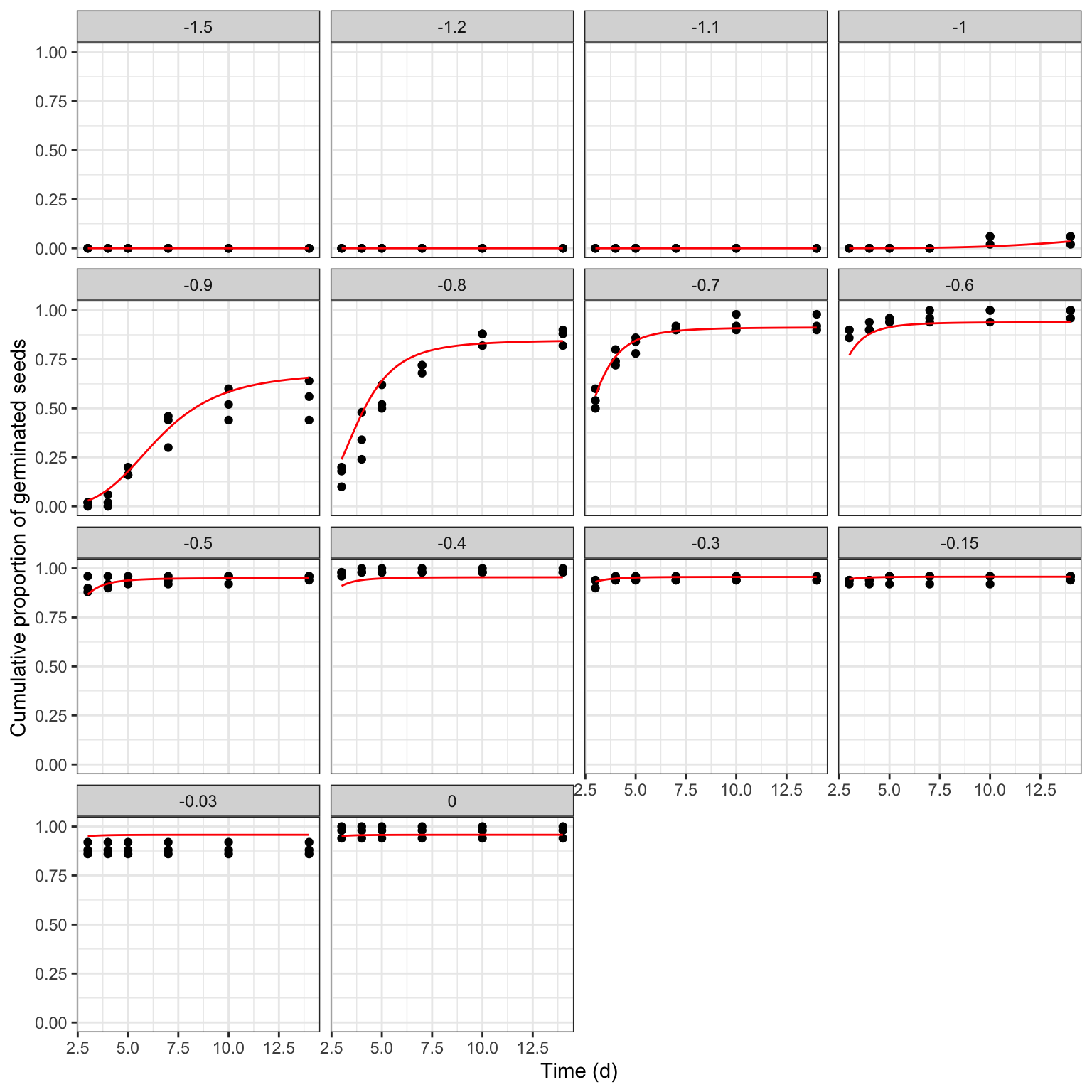

Quantiles for germination times can also be retrieved by using the usual quantile() function, although a single value for base water potential needs to be provided.

quantile(modHTE, probs = c(0.25, 0.50, 0.75), Psi = -0.8)
## 
## Estimated quantiles
## 
##       Estimate       SE
## 1:25%   3.0445 0.091608
## 1:50%   4.1372 0.099117
## 1:75%   6.2726 0.287407

For those who are interested, I give further detail below. Thanks for reading—and don’t forget to check out my new book!

Prof. Andrea Onofri
Department of Agricultural, Food and Environmental Sciences
University of Perugia (Italy)
Send comments to: andrea.onofri@unipg.it

References

1. Bradford, K.J., 2002. Applications of hydrothermal time to quantifying and modeling seed germination and dormancy. Weed Science 50, 248–260.
2. Mesgaran, M.B., Mashhadi, H.R., Alizadeh, H., Hunt, J., Young, K.R., Cousens, R.D., 2013. Importance of distribution function selection for hydrothermal time models of seed germination. Weed Research 53, 89–101. https://doi.org/10.1111/wre.12008
3. Onofri, A., Benincasa, P., Mesgaran, M.B., Ritz, C., 2018. Hydrothermal-time-to-event models for seed germination. European Journal of Agronomy 101, 129–139.
4. Onofri, A., Mesgaran, M.B., Neve, P., Cousens, R.D., 2014. Experimental design and parameter estimation for threshold models in seed germination. Weed Research 54, 425–435. https://doi.org/10.1111/wre.12095
5. Pace, R., Benincasa, P., Ghanem, M.E., Quinet, M., Lutts, S., 2012. Germination of untreated and primed seeds in rapeseed (brassica napus var oleifera del.) under salinity and low matric potential. Experimental Agriculture 48, 238–251.
6. Ritz, C., Jensen, S. M., Gerhard, D., Streibig, J. C. (2019) Dose-Response Analysis Using R CRC Press.

Further detail

Let us conclude this page by briefly describing the remaining models presented by Mesgaran et al. (2013; slightly reparameterised here). For all logarithm-based distributions, \(\delta\) denotes the shifting parameter; indeed, logarithmic distributions are defined only for strictly positive values, whereas water potential typically assumes negative values. The shifting parameter is therefore introduced to translate the cumulative distribution function to the right, allowing negative values of water potential to be accommodated.

Furthermore, for the asymmetric distributions (Gumbel and Weibull distributions), \(\Psi_b\) is replaced by \(\mu\), which represents the location parameter, although it does not necessarily coincide with the median. For all the following distributions, the equations required to derive percentiles of base water potential, such as \(\Psi_{b(25)}\), \(\Psi_{b(50)}\), or \(\Psi_{b(75)}\), are provided below, together with a couple of practical examples of their use.

p <- c(0.25, 0.50, 0.75)
psibs <- coef(mod3)[3] * (-log(-log(p))) + coef(mod3)[2] 
psibs
## [1] -1.0162094 -0.9287760 -0.8178505

predict(mod3, newdata=data.frame(timeAf = Inf, Psi = psibs))
##   timeAf        Psi Prediction
## 1    Inf -1.0162094       0.25
## 2    Inf -0.9287760       0.50
## 3    Inf -0.8178505       0.75

funList <- list(~ sigma * (-log(-log(p))) + mu)
tab <- statforbiology::gnlht(mod3,
                      funList,
                      const = data.frame(p),
                      parameterNames = c("ThetaH", "mu", "sigma"))
tab[,1:4]
##                           Form    p   Estimate          SE
## 1 sigma * (-log(-log(p))) + mu 0.25 -1.0162094 0.009485627
## 2 sigma * (-log(-log(p))) + mu 0.50 -0.9287760 0.008956758
## 3 sigma * (-log(-log(p))) + mu 0.75 -0.8178505 0.009811609

psibs <- exp(-0.347537 * log(-log(p)) + log(-0.985613 + 1.239402)) - 1.239402 

funList <- list(~ exp(-sigma * log(-log(p)) + log(mu + delta)) - delta)
tab <- statforbiology::gnlht(mod5,
                      funList,
                      const = data.frame(p),
                      parameterNames = c("ThetaH", "delta", "mu", "sigma"))
tab[,1:4]
##                                                   Form    p   Estimate
## 1 exp(-sigma * log(-log(p)) + log(mu + delta)) - delta 0.25 -1.0128471
## 2 exp(-sigma * log(-log(p)) + log(mu + delta)) - delta 0.50 -0.9511365
## 3 exp(-sigma * log(-log(p)) + log(mu + delta)) - delta 0.75 -0.8480915
##            SE
## 1 0.007192216
## 2 0.007274446
## 3 0.009085069