Chapter 14 Nonlinear regression
The aim of science is to seek the simplest explanation of complex facts. Seek simplicity and distrust it (A.N. Whitehead)
Biological processes, very rarely follow linear trends. Just think about how a crop grows, or responds to increasing doses of fertilisers/xenobiotics. Or, think about how an herbicide degrades in the soil, or about the germination pattern of a seed population. It is very easy to realise that curvilinear trends, asymptotes and/or inflection points are far more common, in nature. In practice, linear equations in biology are nothing more than a quick way to approximate a response over a very narrow range of the independent variable.
Therefore, we need to be able to fit simple nonlinear models to our experimental data. In this Chapter, we will see how to do this, starting from a simple, but realistic example.
14.1 Case-study: a degradation curve
A soil was enriched with the herbicide metamitron, up to a concentration of 100 ng g1. It was put in 24 aluminium containers, inside a climatic chamber at 20°C. Three containers were randomly selected in eight different times and the residual concentration of metamitron was measured. The observed data are available in the ‘degradation.csv’ file, in an external repository. First of all we load and inspect the data.
fileName <- "https://www.casaonofri.it/_datasets/degradation.csv"
dataset <- read.csv(fileName, header=T)
head(dataset, 10)
##    Time   Conc
## 1     0  96.40
## 2    10  46.30
## 3    20  21.20
## 4    30  17.89
## 5    40  10.10
## 6    50   6.90
## 7    60   3.50
## 8    70   1.90
## 9     0 102.30
## 10   10  49.20
It is always very useful to take a look at the observed data, by plotting the response against the predictor (Figure 14.1); we see that the trend is curvilinear, which rules out the use of simple linear regression.
In order to build a nonlinear regression model, we can use the general form introduced in Chapter 4, that is:
\[Y_i = f(X_i, \theta) + \varepsilon_i\]
where \(X\) is the time, \(Y\) is the concentration, \(f\) is a nonlinear function, \(\theta\) is the set of model parameters and \(\varepsilon\) are the residuals, assumed as independent, gaussian and homoscedastic.
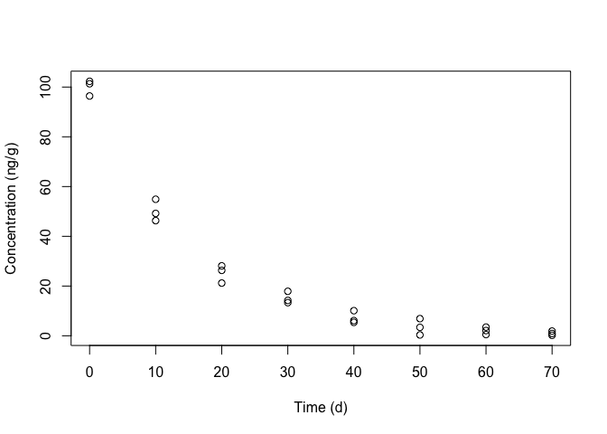
Figure 14.1: Degradation of metamitron in soil
14.2 Model selection
The first task is to select a function \(f\) that matches the observed response shape. You can find full detail elsewhere (go to this link). For now, we can look at Figure 14.2, where we have displayed the shapes of some useful functions for nonlinear regression analysis in agricultural studies. We distinguish:
- Convex/concave shapes (e.g., quadratic polynomial, exponential growth/decay, asymptotic growth, power curve and rectangular hyperbola)
- Sigmoidal shapes (e.g., logistic growth, Gompertz growth and log-logistic dose-response)
- Curves with maxima/minima (e.g., Bragg’s function)
In the above list, the quadratic polynomial is a curvilinear model, but it is linear in the parameters and, therefore, it should have been better included in the previous Chapter about linear regression. However, we decided to include it here, considering its concave shape.
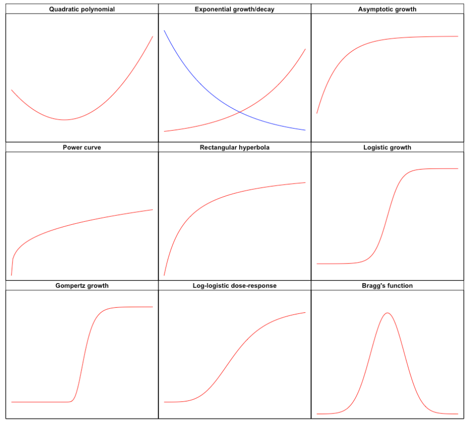
Figure 14.2: The shapes of the most important functions
Behind each of the above shapes, there is a mathematical function, which is shown in Figure 14.3 ).
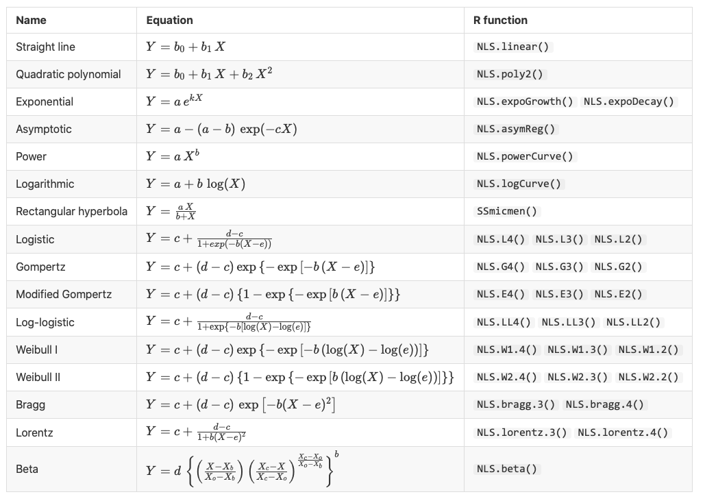
Figure 14.3: Some useful functions for nonlinear regression analysis (equation and R function).
For the dataset under study, considering the shapes in Figure 14.2 and, above all, considering the available literature information, we select an exponential decay equation, with the following form (see also Fig. 14.3 ):
\[Y_i = a \, e^{-k \,X_i} + \varepsilon_i\]
where \(Y\) is the concentration at time \(X\), \(a\) is the initial metamitron concentration and \(k\) is the constant degradation rate.
14.3 Parameter estimation
Now, we have to obtain the least squares estimates of the parameters \(a\) and \(k\). Unfortunately, with nonlinear regression, the least squares problem has no closed form solution and, therefore, we need to tackle the estimation problem in a different way. In general, there are three possibilities
- linearise the nonlinear function;
- approximate the nonlinear function by using a polynomial;
- use numerical methods for the minimisation.
Let’s see advantages and disadvantages of all methods.
14.3.1 Linearisation
In some cases, we can modify the function to make it linear. In this case, we can take the logarithm of both sides and define the following equation:
\[ \log(Y) = \log(A) - k \, X \]
which is, indeed, linear. Therefore, we can take the logarithms of the concentrations and fit a linear model, by using the lm() function:
mod <- lm(log(Conc) ~ Time, data=dataset)
summary(mod)
##
## Call:
## lm(formula = log(Conc) ~ Time, data = dataset)
##
## Residuals:
##      Min       1Q   Median       3Q      Max
## -2.11738 -0.09583  0.05336  0.31166  1.01243
##
## Coefficients:
##              Estimate Std. Error t value Pr(>|t|)
## (Intercept)  4.662874   0.257325   18.12 1.04e-14 ***
## Time        -0.071906   0.006151  -11.69 6.56e-11 ***
## ---
## Signif. codes:  0 '***' 0.001 '**' 0.01 '*' 0.05 '.' 0.1 ' ' 1
##
## Residual standard error: 0.6905 on 22 degrees of freedom
## Multiple R-squared:  0.8613, Adjusted R-squared:  0.855
## F-statistic: 136.6 on 1 and 22 DF,  p-value: 6.564e-11
We see that the slope has a negative sign (the line is decreasing) and the intercept is not the initial concentration value, but its logarithm.
The advantage of this process is that the calculations are very easily performed with every spreadsheet or simple calculator. However, we need to check that the basic assumptions of normal and homoscedastic residuals hold in the logarithmic scale. We do this in the following box.
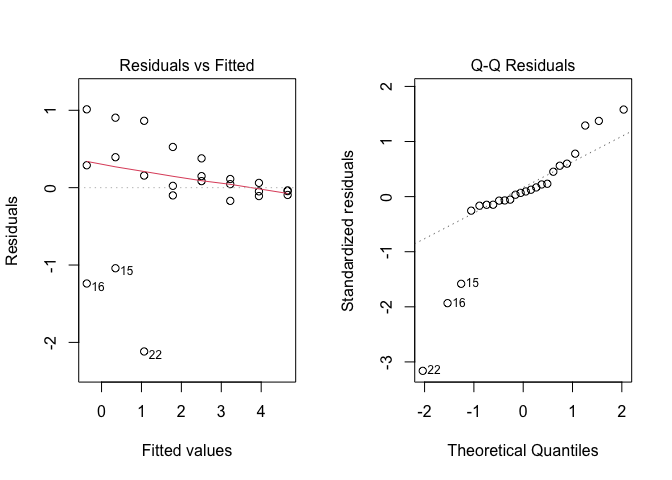
Figure 14.4: Graphical analyses of residuals for nonlinear regression with linearisation of the mean function
The plots show dramatic deviations from homoscedasticity (Figure 14.4 ), which rule out the use of the linearisation method. Please, consider that this conclusion is specific to our dataset, while, in general, the linearisation method can be successfully used, whenever the basic assumptions for linear models appear to hold for the transformed response.
14.3.2 Approximation with a polynomial function
In some other cases, a curvilinear shape can be approximated by using a polynomial equation, that is, indeed, linear in the parameters. In our example, we could think of the descending part of a second order polynomial (see Figure 14.4) and, thus, we fit this model by the usual lm() function:
mod2 <- lm(Conc ~ Time + I(Time^2), data=dataset)
pred <- predict(mod2, newdata = data.frame(Time = seq(0, 70, by = 0.1)))
plot(Conc ~ Time, data=dataset)
lines(pred ~ seq(0, 70, by = 0.1), col = "red")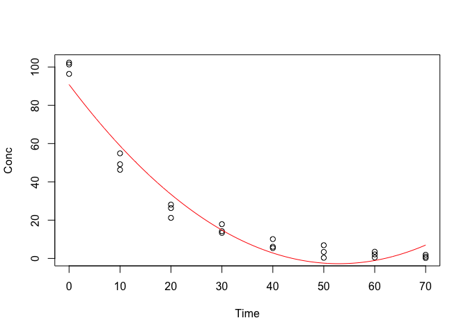
Figure 14.5: Approximating a degradation kinetic by using a second order polynomial
We see that the approximation is good up to 40 days after the beginning of the experiment. Later on, the fitted function appears to deviate from the observed pattern, depicting an unrealistic concentration increase from 55 days onwards (Figure 14.5). Clearly, the use of polynomials may be useful in some other instances, but it not a suitable solution for this case.
14.3.3 Nonlinear least squares
The third possibility consists of using nonlinear least squares, based on the Gauss-Newton iterative algorithm. We need to provide reasonable initial estimates of model parameters and the algorithm updates them, iteratively, until it converges on the approximate least squares solution. Nowadays, thanks to the advent of modern computers, nonlinear least squares have become the most widespread nonlinear regression method, providing very good approximations for most practical needs.
14.4 Nonlinear regression with R
Considering the base R installation, nonlinear least squares regression is implemented in the nls() function. The syntax is very similar to that of the lm() function, although we need to provide reasonable initial values for model parameters. In this case, obtaining such values is relatively easy: \(a\) is the initial concentration and, by looking at the data, we can set this value to 100. The parameter \(k\) is the constant degradation rate, i.e. the percentage daily reduction in concentration; we see that the concentration drops by 50% in ten days, thus we could assume that there is a daily 5% drop (k = 0.05). With such an information, we fit the model, as shown in the box below.
modNlin <- nls(Conc ~ A*exp(-k*Time),
               start=list(A=100, k=0.05),
               data = dataset)
summary(modNlin)
##
## Formula: Conc ~ A * exp(-k * Time)
##
## Parameters:
##    Estimate Std. Error t value Pr(>|t|)
## A 99.634902   1.461047   68.19   <2e-16 ***
## k  0.067039   0.001887   35.53   <2e-16 ***
## ---
## Signif. codes:  0 '***' 0.001 '**' 0.01 '*' 0.05 '.' 0.1 ' ' 1
##
## Residual standard error: 2.621 on 22 degrees of freedom
##
## Number of iterations to convergence: 5
## Achieved convergence tolerance: 4.33e-07
Instead of coding the mean model from the scratch, we can use one of the available self-starting functions (Fig. 14.3 ), which are associated to self-starting routines. This is very useful, as the self-starting functions do not need initial estimates and, thus, we are free from the task of providing them, which is rather difficult for beginners. Indeed, if our initial guesses are not close enough to least squares estimates, the algorithm may freeze during the estimation process and may not reach convergence. Self-starting functions are available within the ‘aomisc’ which needs to be installed from github prior to fitting the model.
14.5 Checking the model
While the estimation of model parameters is performed by using numerical methods, checking a fitted model is done by using the very same methods as shown for simple linear regression, with slight differences. In the following section we will show some of the R methods for nonlinear models, which can be used on ‘nls’ objects.
14.5.1 Graphical analyses of residuals
First of all, we check the basic assumptions of normality and homoscedasticity of model residuals, by the usual diagnostic plots. We can us the plotnls() function, as available in the ‘aomisc’ package.
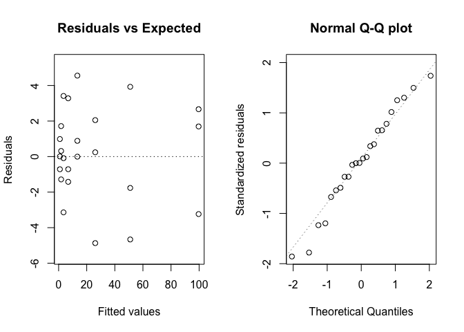
Figure 14.6: Graphical analyses of residuals relating to the degradation of metamitron in soil.
Figure 14.6 does not show any visible deviations and, thus, we proceed to plotting the observed data along with model predictions (Figure 14.7), e.g., by using the plotnls() function, in the ‘aomisc’ package.
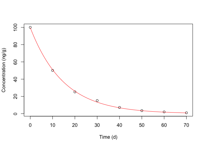
Figure 14.7: Degradation kinetic for metamitron in soil: symbols show the observed data, the red line shows the fitted equation
14.5.2 Approximate F test for lack of fit
If we have replicates, we can fit an ANOVA model and compare this latter model to the nonlinear regression model, as we have already shown in Chapter 13, for linear regression models (F test for lack of fit). With R, this test can be performed by using the anova() method and passing the two model objects as arguments. The box below shows that the null hypothesis of no lack of fit can be accepted.
14.5.3 The coefficient of determination (R2)
The R2 coefficient in nonlinear regression should not be used as a measure of goodness of fit, because it represents the ratio between the residual deviances for the model under comparison and for a model with the only intercept (see previous chapter). Some non-linear models do not have an intercept and, therefore, the R2 value is not meaningful and can also assume values outside the range from 0 to 1.
Such an argument can be, at least partly, overcame by using the Pseudo R2 (Schabenberger and Pierce, 2002), that is the proportion of variance explained by the regression effect:
\[R_a^2 = 1 - \frac{MSE}{MST}\]
where MSE is the residual mean square and MST is total mean square. For our example:
Whenever necessary, The Pseudo-R2 value can be obtained by using the R2nls() function, in the ‘aomisc’ package, as shown in the box below.
14.6 Stabilising transformations
In some cases, it may happen that the model does not fit the data (lack of fit) or that the residuals are not gaussian and homoscedastic. In the first case, we have to discard the model and select a new one, that fits better to the observed data.
In the other cases (heteroscedastic or non-normal residuals), similarly to linear regression, we should adopt some sort of stabilising transformations, possibly selected by using the Box-Cox method. However, nonlinear regression poses an additional issue, that we should keep into account. Indeed, in most cases, the parameters of nonlinear models are characterised by a clear biological meaning, such as, for example, the parameter \(a\) in the exponential equation above, that is the initial concentration value. If we transform the response into, e.g., its logarithm, the estimated \(a\) represents the logarithm of the initial concentration and its biological meaning is lost.
In order to avoid such a problem and obtain parameter estimates in their original scale, the ‘transform-both-sides’ approach is feasible, where we use the Box-Cox family of transformations (see Chapter 8) to transform both the response and the model:
\[Y_i^\lambda = f(X_i)^\lambda + \varepsilon_i\]
In order to use this technique in R, we can use the boxcox.nls() method in the ‘aomisc’ package, that is very similar to the ‘boxcox()’ method in the MASS package (see Chapter 8). The boxcox.nls() method returns the maximum likelihood value for \(\lambda\) with confidence intervals and a likelihood graph as a function of \(\lambda\) can also be obtained by using the argument ‘plotit = T’

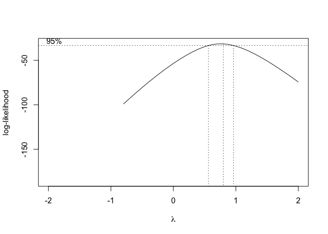
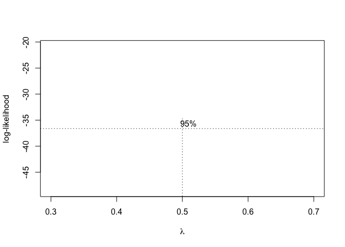
Figure 14.8: Selection of the ‘lambda’ value for the Box-Cox transformation of a nonlinear regression model
From Figure 14.8, we see that the transformation is not required, although a value \(\lambda\) = 0.5 (square-root transformation; see previous chapter) might be used to maximise the likelihood of the data under the selected model. We can specify our favourite \(\lambda\) value and get the corresponding fit by using the same boxcox.nsl() function and passing an extra-argument, as shown in the box below.
summary(modNlin3)
##
## Estimated lambda: 0.5
## Confidence interval for lambda: [NA,NA]
##
## Formula: newRes ~ eval(parse(text = newFormula), df)
##
## Parameters:
##    Estimate Std. Error t value Pr(>|t|)
## A 99.532761   4.625343   21.52 2.87e-16 ***
## k  0.067068   0.002749   24.40  < 2e-16 ***
## ---
## Signif. codes:  0 '***' 0.001 '**' 0.01 '*' 0.05 '.' 0.1 ' ' 1
##
## Residual standard error: 0.9196 on 22 degrees of freedom
##
## Number of iterations to convergence: 1
## Achieved convergence tolerance: 7.541e-06
We see that, in spite of the stabilising transformation, the estimated parameters have not lost their measurement unit.
14.7 Making predictions
As shown for linear regression in Chapter 13, every fitted model can be used to make predictions, i.e. to calculate the response for a given X-value or to calculate the X-value corresponding to a given response.
Analogously to linear regression, we could make predictions by using the predict() method, although, for nonlinear regression objects, this method does not return standard errors. Therefore, we can use the gnlht() function in the ‘aomisc’ package, which requires the following arguments:
- a list of functions containing model parameters (with the same names as the fitted model) and, possibly, some other parameters
- if the previous function contain further parameters with respect to the fitted model, their values need to be given in a data frame as an extra-argument
In the box below we make predictions for the response at 5, 10 and 15 days after the beginning of the experiment.
func <- list(~A * exp(-k * time))
const <- data.frame(time = c(5, 10, 15))
gnlht(modNlin, func,  const)
##                 Form time Estimate        SE  t-value      p-value
## 1 A * exp(-k * time)    5 71.25873 0.9505532 74.96553 5.340741e-28
## 2 A * exp(-k * time)   10 50.96413 0.9100611 56.00078 3.163518e-25
## 3 A * exp(-k * time)   15 36.44947 0.9205315 39.59611 6.029672e-22
The same method can be used to make inverse predictions. In our case, the inverse function is:
\[X = - \frac{log \left( \frac{Y}{A} \right)}{k}\]
We can calculate the times required for the concentration to drop to, e.g., 10 and 20 mg/g by using the code in the following box.
func <- list(~ -(log(Conc/A)/k))
const <- data.frame(Conc = c(10, 20))
gnlht(modNlin, func,  const)
##               Form Conc Estimate        SE  t-value      p-value
## 1 -(log(Conc/A)/k)   10 34.29237 0.8871429 38.65484 1.016347e-21
## 2 -(log(Conc/A)/k)   20 23.95291 0.6065930 39.48761 6.399715e-22
In the same fashion, we can calculate the half-life (i.e. the time required for the concentration to drop to half of the initial value), by considering that:
\[t_{1/2} = - \frac{ \log \left( {\frac{1}{2}} \right) }{k}\]
The code is::
func <- list(~ -(log(0.5)/k))
gnlht(modNlin, func)
##            Form Estimate       SE t-value      p-value
## 1 -(log(0.5)/k) 10.33945 0.291017 35.5287 6.318214e-21
The ‘gnlht()’ function provides standard errors based on the delta method, which we have already introduced in a previous chapter.
14.8 Further readings
- Bates, D.M., Watts, D.G., 1988. Nonlinear regression analysis & its applications. John Wiley & Sons, Inc., Books.
- Bolker, B.M., 2008. Ecological models and data in R. Princeton University Press, Books.
- Carroll, R.J., Ruppert, D., 1988. Transformation and weighting in regression. Chapman and Hall, Books.
- Ratkowsky, D.A., 1990. Handbook of nonlinear regression models. Marcel Dekker Inc., Books.
- Ritz, C., Streibig, J.C., 2008. Nonlinear regression with R. Springer-Verlag New York Inc., Books.
- Schabenberger, O., Pierce, F.J., 2002. Contemporary statistical models for the plant and soil sciences. Taylor & Francis, CRC Press