Chapter 11 Multi-way ANOVA models with interactions
A theory is just a mathematical model to describe the observations (K. Popper)
In the previous Chapter we have seen models with more than one explanatory factor, that are used to describe data from Randomised Complete Block Designs and Latin Square designs, where we have one treatment factor and, respectively, one or two blocking factors. Most often, with these designs we have only one value for each combination between the experimental factor and the blocking factor; e.g., there is usually only one observation per treatment in each block in a Randomised Complete Block Design.
In this Chapter, we would like to introduce a new situation, where we have more than one experimental factor and more than one observation for each combination of factor levels. In Chapter 2, we have already seen an example where we compared three tillage levels and two weed control methods in a crossed factorial design and we had four replicates for each combination of tillage and weed control method. In such condition, we can obtain an estimate of the so-called interaction between experimental factors, which is a very relevant information.
11.1 The ‘interaction’ concept
Let’s look at the Figure 11.1 where we displayed three possible situations, relating to the combinations between the factor A, with two levels (A1 and A2) and the factor B with two levels (B1 and B2). Each symbol represents a combination; e.g., in the left panel we see that the A1B1 combination showed a response equal to 10, while the A2B1 combination showed a response equal to 14. Therefore, passing from A1 to A2 gave an effect of +4 units. Likewise, we see that the yield of A1B2 was 15 and, thus, passing from B1 to B2 gave an effect of +5 units. Accordingly, we can predict the yield of A2B2 by summing up the yield of A1B1, the effact of passing from A1 to A2 and the effect of passing from B1 to B2, i.e. \(10 + 4 + 5 = 19\). In this case A and B do not interact to each other and their effects are simply additive.
Now, let’s look at the central panel. Passing from A1B1 to A2B1 and passing from A1B1 to A1B2 produced the same effects as in the previous case (respectively +4 and +5 units), but we can no longer predict the response of A2B2, as we see that, while the expected value is 19, the observed value is 16. There must be some effect that hinders the response of this specific combination A2B2 and such an effect is known as the interaction between the factors A and B (or ‘A \(\times\) B’ interaction). We can quantify such an interaction effect as \(16 - 19 = -3\) units; this is an example of negative interaction, as the observed response is lower than the expected response. Furthermore, this is an example of simple interaction, where the expected response is lower, but the ranking of treatments is not affected; indeed, A2 is always higher than A1, regardless of B and B1 is always lower than B2, regardless of A.
If we look at the left panel, we see that the interaction effect is even more dramatic: for A2B2 we observe 9 instead of 19, which means that the interaction is -10 units and it causes the change of ranking: A2 is higher than A1 when B is equal to B1, while the ranking is reversed when B is equal to B2. Whenever the interaction effect modifies the ranking of treatments, we talk about cross-over interaction.
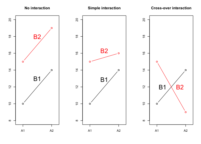
Figure 11.1: Possible relationships between experimental factors
Why are we so concerned by the interaction? Let’s take a further look at the third situation, as seen in the left panel of Figure 11.1. Table 11.1 shows the means for the four combinations (A1B1, A1B2, A2B1, A2B2) that are usually named cell means, together with the means for main factor levels (A1, A2, B1 and B2), usually named marginal means, and the overall mean.
| B1 | B2 | Average | |
|---|---|---|---|
| A1 | 10.0 | 14.0 | 12.0 |
| A2 | 15.0 | 9.0 | 12.0 |
| Average | 12.5 | 11.5 | 12.0 |
If we look at the marginal means, we would have the wrong impression that factor A is totally ineffective and factor B only gives a minor effect. Indeed, both factors have very wide effects, although they are masked by the presence of a cross-over interaction.
That is why we are so much concerned about possible interactions between the experimental factors: these effects can be highly misleading when we look at the marginal effects of A and B. And this is also why we organise a factorial experiment, instead of making two separate experiments for A and for B.
11.2 Genotype by N interactions
We will use an example relating to a genotype experiment, where 5 winter wheat genotypes were compared at two different nitrogen fertilisation levels, according to a RCBD, with 3 replicates. The aim of such an experiment was to assess whether the ranking of genotypes, and thus genotype recommendation, is affected by N availability. The dataset was generated by Monte Carlo methods, starting from the results reported in Stagnari et al. (2013) and it was cut to five genotypes instead of the original 15 to make the hand-calculations easier.
Yield results are reported in the file ‘NGenotype.csv’, that is available in the usual online repository. After loading the file we transform the numeric explanatory variables into factors.
filePath <- "https://www.casaonofri.it/_datasets/"
fileName <- "NGenotype.csv"
file <- paste(filePath, fileName, sep = "")
dataset <- read.csv(file, header=T)
dataset$Block <- factor(dataset$Block)
dataset$N <- factor(dataset$N)
head(dataset, 10)
##    Block Genotype N Yield
## 1      1        A 1 2.146
## 2      2        A 1 2.433
## 3      3        A 1 2.579
## 4      1        A 2 2.362
## 5      2        A 2 2.919
## 6      3        A 2 2.912
## 7      1        B 1 2.935
## 8      2        B 1 2.919
## 9      3        B 1 2.892
## 10     1        B 2 3.241
11.2.1 Model definition
Yield results are determined by four effects:
- blocks
- genotypes
- N levels
- ‘genotype \(\times\) N’ interaction
Accordingly, a linear model can be written as:
\[Y_{ijk} = \mu + \gamma_k + \alpha_i + \beta_j + \alpha\beta_{ij} + \varepsilon_{ijk}\]
where \(\mu\) is the intercept, \(\gamma_k\) is the effect of the \(k\)th block, \(\alpha_i\) is the effect of the \(i\)th genotype, \(\beta_j\) is the effect of the \(j\)th N level and \(\alpha\beta_{ij}\) is the interaction effect of the combination between the \(i\)th genotype and \(j\)th nitrogen level. The unknown random effects are represented by the residuals \(\varepsilon_{ijk}\), which we assume as gaussian distributed and homoscedastic, with mean equal to 0 and standard deviation equal to \(\sigma\).
11.2.2 Model fitting by hand
As in previous chapters, we will show how we can fit an ANOVA model by hand, as this is the best way to understand this technique; you can safely skip this part. if you are only interested in learning how to fit models with a computer.
Model fitting by hand is most easily perfomed by using the sum-to-zero constraint and the method of moments, although I have to remind that this latter method is only valid with balanced data.
First of all, we calculate all means: for blocks, genotypes, N levels and for the combinations between genotypes and nitrogen levels. We use the tapply() function, which, for the case of the ‘genotype by nitrogen’ combinations, returns a matrix.
mu <- mean(dataset$Yield)
bMean <- tapply(dataset$Yield, dataset$Block, mean)
gMean <- tapply(dataset$Yield, dataset$Genotype, mean)
nMean <- tapply(dataset$Yield, dataset$N, mean)
gnMean <- tapply(dataset$Yield, list(dataset$Genotype,dataset$N), mean)
mu
## [1] 2.901967
bMean
##      1      2      3
## 2.7997 2.9586 2.9476
gMean
##        A        B        C        D        E
## 2.558500 3.077333 2.362167 3.151000 3.360833
gnMean
##          1        2
## A 2.386000 2.731000
## B 2.915333 3.239333
## C 2.533333 2.191000
## D 2.956000 3.346000
## E 3.256000 3.465667
With the sum-to-zero constraint, the effects are differences of group means with respect to the overall mean. Therefore, we can calculate \(\gamma\), \(\alpha\) and \(\beta\), as follows:
gamma <- bMean - mu
alpha <- gMean - mu
beta <- nMean - mu
gamma
##           1           2           3
## -0.10226667  0.05663333  0.04563333
alpha
##          A          B          C          D          E
## -0.3434667  0.1753667 -0.5398000  0.2490333  0.4588667
beta
##           1           2
## -0.09263333  0.09263333
Now, as the average block effect is constrained to be zero (sum-to-zero contraint), the mean for a ‘genotype by nitrogen’ combination is equal to:
\[\bar{Y}_{ij.} = \mu + \alpha_i + \beta_j + \alpha\beta_{ij}\]
From there, we obtain the interaction effect as:
\[\alpha\beta_{ij} = \bar{Y}_{ij.} - \mu - \alpha_i - \beta_j\]
that is:
alphaBeta <- gnMean - mu - matrix(rep(alpha, 2), 5, 2) -
  matrix(rep(beta, 5), 5, 2, byrow = T)
alphaBeta
##             1           2
## A -0.07986667  0.07986667
## B -0.06936667  0.06936667
## C  0.26380000 -0.26380000
## D -0.10236667  0.10236667
## E -0.01220000  0.01220000
For example, the interaction effects for the first combination (genotype A and first nitrogen rate) is \(-0.07986667\), while for the second combination (genotype B and first nitrogen rate) the interaction effect is \(-0.06936667\). Indeed, both combinations produce less than expected under addivity.
gnMean - mu - matrix(rep(alpha, 2), 5, 2) -
  matrix(rep(beta, 5), 5, 2, byrow = T)
##             1           2
## A -0.07986667  0.07986667
## B -0.06936667  0.06936667
## C  0.26380000 -0.26380000
## D -0.10236667  0.10236667
## E -0.01220000  0.01220000
With little patience, we can easily complete the calculations by hand and organise them in a summary data frame, together with the expected values (i.e. the sums \(\hat{Y}_{ijk} = \mu + \gamma_k + \alpha_i + \beta_j + \alpha\beta_{ij}\)) and the residuals (i.e. the differences between the observed and the expected values). You can use the prospect below to check your calculations.
print(tab, digits = 3)
##    Block Genotype N Yield  mu   gamma  alpha    beta alphaBeta
## 1      1        A 1  2.15 2.9 -0.1023 -0.343 -0.0926   -0.0799
## 2      2        A 1  2.43 2.9  0.0566 -0.343 -0.0926   -0.0799
## 3      3        A 1  2.58 2.9  0.0456 -0.343 -0.0926   -0.0799
## 4      1        A 2  2.36 2.9 -0.1023 -0.343  0.0926    0.0799
## 5      2        A 2  2.92 2.9  0.0566 -0.343  0.0926    0.0799
## 6      3        A 2  2.91 2.9  0.0456 -0.343  0.0926    0.0799
## 7      1        B 1  2.94 2.9 -0.1023  0.175 -0.0926   -0.0694
## 8      2        B 1  2.92 2.9  0.0566  0.175 -0.0926   -0.0694
## 9      3        B 1  2.89 2.9  0.0456  0.175 -0.0926   -0.0694
## 10     1        B 2  3.24 2.9 -0.1023  0.175  0.0926    0.0694
## 11     2        B 2  3.30 2.9  0.0566  0.175  0.0926    0.0694
## 12     3        B 2  3.17 2.9  0.0456  0.175  0.0926    0.0694
## 13     1        C 1  2.38 2.9 -0.1023 -0.540 -0.0926    0.2638
## 14     2        C 1  2.53 2.9  0.0566 -0.540 -0.0926    0.2638
## 15     3        C 1  2.69 2.9  0.0456 -0.540 -0.0926    0.2638
## 16     1        C 2  2.30 2.9 -0.1023 -0.540  0.0926   -0.2638
## 17     2        C 2  2.19 2.9  0.0566 -0.540  0.0926   -0.2638
## 18     3        C 2  2.08 2.9  0.0456 -0.540  0.0926   -0.2638
## 19     1        D 1  2.69 2.9 -0.1023  0.249 -0.0926   -0.1024
## 20     2        D 1  3.34 2.9  0.0566  0.249 -0.0926   -0.1024
## 21     3        D 1  2.84 2.9  0.0456  0.249 -0.0926   -0.1024
## 22     1        D 2  3.30 2.9 -0.1023  0.249  0.0926    0.1024
## 23     2        D 2  3.29 2.9  0.0566  0.249  0.0926    0.1024
## 24     3        D 2  3.45 2.9  0.0456  0.249  0.0926    0.1024
## 25     1        E 1  3.24 2.9 -0.1023  0.459 -0.0926   -0.0122
## 26     2        E 1  3.06 2.9  0.0566  0.459 -0.0926   -0.0122
## 27     3        E 1  3.46 2.9  0.0456  0.459 -0.0926   -0.0122
## 28     1        E 2  3.41 2.9 -0.1023  0.459  0.0926    0.0122
## 29     2        E 2  3.60 2.9  0.0566  0.459  0.0926    0.0122
## 30     3        E 2  3.38 2.9  0.0456  0.459  0.0926    0.0122
##    residuals
## 1   -0.13773
## 2   -0.00963
## 3    0.14737
## 4   -0.26673
## 5    0.13137
## 6    0.13537
## 7    0.12193
## 8   -0.05297
## 9   -0.06897
## 10   0.10393
## 11   0.00803
## 12  -0.11197
## 13  -0.05407
## 14  -0.06097
## 15   0.11503
## 16   0.20827
## 17  -0.05663
## 18  -0.15163
## 19  -0.16873
## 20   0.32837
## 21  -0.15963
## 22   0.05527
## 23  -0.11563
## 24   0.06037
## 25   0.08927
## 26  -0.24963
## 27   0.16037
## 28   0.04860
## 29   0.07770
## 30  -0.12630
The table above shows all effects and permits the calculation of sum of squares, as the sums of the squared elements in each column. The residual sum of squares is:
while the sum of squares for blocks, genotype, nitrogen and interaction effects are calculated as:
BSS <- sum(tab$gamma ^ 2)
BSS
## [1] 0.1574821
GSS <- sum(tab$alpha ^ 2)
GSS
## [1] 4.276098
NSS <- sum(tab$beta ^ 2)
NSS
## [1] 0.257428
GNSS <- sum(tab$alphaBeta ^ 2)
GNSS
## [1] 0.5484518
Also in this case, we can see that the sum of all the above mentioned sum of squares is equal to the total deviance of all the observations.
We clearly see that the whole variability of yield has been partitioned in four parts, one is due to the effect of blocks, another one is due to the effect of genotypes, another one is due to the effect of N fertilisation and, finally, the last one is due to all other unknown effects of random nature.
It is no worth to keep on with manual calculations from now on, thus let’s switch the computer on.
11.2.3 Model fitting with R
Model fitting with R is exactly the same as shown in previous chapters: we need to include all effect, as well as the interaction, which is represented by using the colon indicator ‘:’. Therefore, model syntax is:
Yield ~ Block + Genotype + N + Genotype:Nwhich can be abbreviated as:
Yield ~ Block + Genotype * NThe full coding is:
Before, proceeding, we need to perform the usual graphical check of model residuals, that is reported in Figure 11.2.
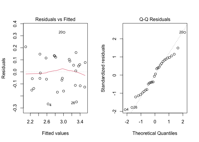
Figure 11.2: Graphical analyses of residuals for a two-way ANOVA model with replicates
From the graph, we see no evident deviations from the basic assumptions for linear models: variances do not seem to be dependent on the expected values and the QQ-plot does not show any relevant deviation from the diagonal. Therefore, we proceed to data analyses with no further checks.
With ANOVA models we are not very much interested in parameter estimates and, therefore, we proceed to variance partitioning, by using the anova() method.
anova(mod)
## Analysis of Variance Table
##
## Response: Yield
##            Df Sum Sq Mean Sq F value   Pr(>F)
## Block       2 0.1575 0.07874  2.4228  0.11701
## Genotype    4 4.2761 1.06902 32.8936 4.72e-08 ***
## N           1 0.2574 0.25743  7.9210  0.01148 *
## Genotype:N  4 0.5485 0.13711  4.2189  0.01392 *
## Residuals  18 0.5850 0.03250
## ---
## Signif. codes:  0 '***' 0.001 '**' 0.01 '*' 0.05 '.' 0.1 ' ' 1
We see that the sum of squares are the same as those obtained by hand-calculations, while the degrees of freedom are easily obtained as the number of blocks/genotypes/N levels minus one. As for the interaction, the number of degrees of freedom is given by the product of the number of genotypes minus one and the number of nitrogen levels minus 1 (\(4 \times 1 = 4\)). The number of degrees of freedom for the residuals is obtained by subtraction, considering that the total number of degrees of freedom for 30 yield data is 29. Therefore, the residual sum of squares has \(29 - 2 - 4 - 1 - 4 = 18\) degrees of freedom.
The variances are obtained by dividing the mean squares for the respective number of degrees of freedom; These variances can be compared with the residual variance by three F ratios, which are, 2.42, 32.9, 7.9 and 4.2, respectively for the blocks, genotypes, N levels and ‘genotype by nitrogen’ interaction.
Apart from the block effects, which are uninteresting from a biological point of view, it is relevant to ask whether the other effects are significant. We know that the sampling distribution for the F ratio under the null hypothesis is Fisher-Snedecor, with the appropriate number of degrees of freedom. For example, for the genotype effect, the sampling distribution is Fisher-Snedecor with 4 degrees of freedom at the numerator and 18 degrees of freedom at the denominator. The probability of observing a value of 32.9 or higher under the null hypothesis is:
This is exactly the result reported in the ANOVA table above, together with the P-levels for all other effects.
Reading the P-levels for a two-way ANOVA requires some care and it is fundamental to proceed from bottom to top. Indeed, a significant interaction makes the P-level for main effects irrelevant, as their significance may be hidden by the presence of cross-over interaction. We have seen an example of such a situation at the beginning of this Chapter.
11.2.4 Inferences and standard errors
Standard errors for means and differences are calculated by the usual rule, starting from the residual standard deviation, that is the square root of the residual variance. In R we can use the ‘sigma’ slot in the ‘summary(mod)’ object:
We know that we have to divide the above amount for the square root of the number of replicates, but we have to carefully consider this latter information. Indeed, the combinations of factor levels have three replicates (\(r = 3\)), but, for each genotype, there is a higher number of replicates, given by the product of \(r\) by the number of N levels (\(3 \times 2 = 6\)). On the other hand, for each N level, we have \(r \times 5 = 15\) replicates, where 5 is the number of genotypes (take a look at the dataset to confirm this). Therefore, the SEMs, respectively for genotype means, N level means and the combinations, are:
\[SEM_g = \frac{0.1802761}{\sqrt{3 \cdot 2}} = 0.0736\]
\[SEM_n = \frac{0.1802761}{\sqrt{3 \cdot 5}} = 0.0465\]
\[SEM_{gn} = \frac{1.87}{\sqrt{3}} = 0.104\]
We may note that the means for main effects are estimated with higher precision, owing to the higher number of replicates.
Standard errors for the differences between means can be easily derived by multiplying the SEMs for \(\sqrt{2}\) as we have shown in previous Chapters.
11.2.5 Expected marginal means
In general, with nominal explanatory variables we are interested in presenting and commenting the means. In this case, apart from the blocks, we have three types of means to consider:
- the marginal means for genotypes
- the marginal means for N fertilisation levels
- the cell means for the combinations of genotype and N fertilisation levels
We have already calculated the arithmetic means, although expected marginal means are generally preferable, as they are equal to the arithmetic means when the data is balanced, but they are more reliable than arithmetic means when the data is unbalanced. Expected marginal means can be obtained with the emmeans() function in the ‘emmeans’ package, although we need to be careful in selecting which means to present
As a general rule, for the reasons given above, we recommend that the means for the combinations are always reported in presence of a significant interaction, while the means for main effects can be reported and commented when the interaction is not significant. In the code below we added a letter display, following pairwise comparisons with multiplicity adjustment.
library(emmeans)
GNmeans <- emmeans(mod, ~Genotype:N)
multcomp::cld(GNmeans, Letters=LETTERS)
##  Genotype N emmean    SE df lower.CL upper.CL .group
##  C        2   2.19 0.104 18     1.97     2.41  A
##  A        1   2.39 0.104 18     2.17     2.60  AB
##  C        1   2.53 0.104 18     2.31     2.75  ABC
##  A        2   2.73 0.104 18     2.51     2.95   BCD
##  B        1   2.92 0.104 18     2.70     3.13    CDE
##  D        1   2.96 0.104 18     2.74     3.17    CDEF
##  B        2   3.24 0.104 18     3.02     3.46     DEF
##  E        1   3.26 0.104 18     3.04     3.47     DEF
##  D        2   3.35 0.104 18     3.13     3.56      EF
##  E        2   3.47 0.104 18     3.25     3.68       F
##
## Results are averaged over the levels of: Block
## Confidence level used: 0.95
## P value adjustment: tukey method for comparing a family of 10 estimates
## significance level used: alpha = 0.05
## NOTE: If two or more means share the same grouping symbol,
##       then we cannot show them to be different.
##       But we also did not show them to be the same.
In the above output, multiplicity correction has been made for \(10 \time 9 / 2 = 45\) comparisons. If we were only interested in comparing, e.g., the genotypes within each N level, we would have a lower number of comparisons (\(5 \times 4/2 \times 2 = 20\)) and, consequently, we would need a lower degree of multiplicity correction. We can specify such an analysis by using the following code (please note the use of the nesting operator ‘|’).
GNmeans2 <- emmeans(mod, ~Genotype|N)
multcomp::cld(GNmeans2, Letters=LETTERS)
## N = 1:
##  Genotype emmean    SE df lower.CL upper.CL .group
##  A          2.39 0.104 18     2.17     2.60  A
##  C          2.53 0.104 18     2.31     2.75  AB
##  B          2.92 0.104 18     2.70     3.13   BC
##  D          2.96 0.104 18     2.74     3.17   BC
##  E          3.26 0.104 18     3.04     3.47    C
##
## N = 2:
##  Genotype emmean    SE df lower.CL upper.CL .group
##  C          2.19 0.104 18     1.97     2.41  A
##  A          2.73 0.104 18     2.51     2.95   B
##  B          3.24 0.104 18     3.02     3.46    C
##  D          3.35 0.104 18     3.13     3.56    C
##  E          3.47 0.104 18     3.25     3.68    C
##
## Results are averaged over the levels of: Block
## Confidence level used: 0.95
## P value adjustment: tukey method for comparing a family of 5 estimates
## significance level used: alpha = 0.05
## NOTE: If two or more means share the same grouping symbol,
##       then we cannot show them to be different.
##       But we also did not show them to be the same.
From the table above, we note that the ranking of genotypes is strongly dependent on N fertilisation (C is better than A with N = 2, while it is not significantly different with A = 1), which is explained by the presence of cross-over interaction.
11.3 Nested effects: maize crosses
In the previous example the factorial design was fully crossed, as the genotypes were the same for both N fertilisation levels. In plant breeding, it is fairly common to find nested designs, where the levels of one factor change depending on the levels of the other factor. For example, we could take three maize pollinating inbreds (A1, A2 and A3) and cross them with three female inbred lines (B1, B2 and B3 crossed with A1, B4, B5 and B6 crossed with A2 and B7, B8 and B9 crossed with A3). In the end, we harvest the yield of nine hybrids in three groups, depending on the pollinating line.
The dataset ‘crosses.csv’ reports the results of a similar experiments, designed as complete blocks with 4 replicates (36 values, in total) and online available, in the usual web repository.
dataset <- read.csv("https://www.casaonofri.it/_datasets/crosses.csv", header=T)
head(dataset, 15)
##    Male Female Block     Yield
## 1    A1     B1     1  9.984718
## 2    A1     B1     2 13.932663
## 3    A1     B1     3 12.201312
## 4    A1     B1     4  1.916661
## 5    A1     B2     1  8.928465
## 6    A1     B2     2 10.513908
## 7    A1     B2     3 10.035964
## 8    A1     B2     4  2.375822
## 9    A1     B3     1 21.511028
## 10   A1     B3     2 21.859852
## 11   A1     B3     3 17.626284
## 12   A1     B3     4 13.966646
## 13   A2     B4     1 17.483089
## 14   A2     B4     2 19.480893
## 15   A2     B4     3 12.838792
11.3.1 Model definition
In this experiment, the yield variation can be described as a function of the blocks (\(\gamma\)) and ‘father’ effect (\(\alpha\)), while ‘mother’ effect (\(\delta\)) can only be determined within each male line, as the female lines are different for each male line. In other words, the ‘mother’ effect is nested within the ‘father’ effect, as shown in Figure 11.3. The linear model is as follows:
\[Y_{ijk} = \mu + \gamma_k + \alpha_i + \delta_{ij} + \varepsilon_{ijk}\]
where \(\gamma_k\) is the block effect (\(k\) goes from 1 to 4), \(\alpha_i\) is the ‘father’ effect (\(i\) goes from 1 to 3) and \(\delta_{ij}\) is the ‘mother’ effect (\(j\) goes from 1 to 9) within each male line \(i\). The random component \(\varepsilon\) is assumed as gaussian and homoscedastic, with mean equal to 0 and standard deviation equal to \(\sigma\).
Hopefully, the difference from the above model and a model for a two-way factorial design is clear: while this latter model contains the two main effects A and B and their interaction A:B, a model for a nested design contains only the main effect for A and the effect of B within A (A/B), while the main effect B is missing, as it does not exist, in practice.
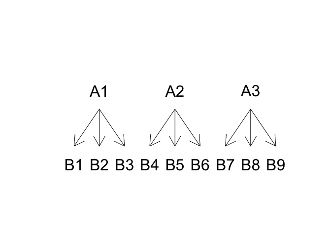
Figure 11.3: Structure for a nested design
11.3.2 Parameter estimation
In this case, we use R for the estimation of model parameters; as shown below, the model formula does not contain the main female effect.
As usual, before proceedin,g we inspect the residuals, by using the plot() method. The Figure 11.4 shows no visible problems with basic assumptions and, therefore, we proceed to variance partitioning.
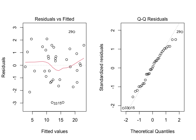
Figure 11.4: Graphical analyses of residuals for a two-way nested ANOVA model with replicates
anova(mod)
## Analysis of Variance Table
##
## Response: Yield
##               Df Sum Sq Mean Sq F value    Pr(>F)
## factor(Block)  3 383.75 127.917  44.355 6.051e-10 ***
## Male           2 134.76  67.378  23.363 2.331e-06 ***
## Male:Female    6 575.16  95.860  33.239 1.742e-10 ***
## Residuals     24  69.21   2.884
## ---
## Signif. codes:  0 '***' 0.001 '**' 0.01 '*' 0.05 '.' 0.1 ' ' 1
From the ANOVA table we see that all effects are significant; as before, we should read the ANOVA table from bottom up and we should consider that the main affect of ‘father’ is relatively unimportant, as the three lines are mated to different female lines.
We can use the function ‘emmeans()’ to calculate the expected marginal means and compare them.
library(emmeans)
mfMeans <- emmeans(mod, ~Female|Male)
multcomp::cld(mfMeans, Letters = LETTERS)
## Male = A1:
##  Female emmean    SE df lower.CL upper.CL .group
##  B2       7.96 0.849 24     6.21     9.72  A
##  B1       9.51 0.849 24     7.76    11.26  A
##  B3      18.74 0.849 24    16.99    20.49   B
##
## Male = A2:
##  Female emmean    SE df lower.CL upper.CL .group
##  B6       8.72 0.849 24     6.97    10.47  A
##  B5      11.23 0.849 24     9.48    12.98  AB
##  B4      15.18 0.849 24    13.43    16.93   B
##
## Male = A3:
##  Female emmean    SE df lower.CL upper.CL .group
##  B9      10.11 0.849 24     8.35    11.86  A
##  B8      17.73 0.849 24    15.97    19.48   B
##  B7      20.12 0.849 24    18.36    21.87   B
##
## Results are averaged over the levels of: Block
## Confidence level used: 0.95
## Results are averaged over some or all of the levels of: Block
## P value adjustment: tukey method for comparing a family of 9 estimates
## significance level used: alpha = 0.05
## NOTE: If two or more means share the same grouping symbol,
##       then we cannot show them to be different.
##       But we also did not show them to be the same.
In conclusion, we see that the analyses of nested factorial experiments is almost the same as for fully crossed factorial experiments, with the only exception that the main effect for the ‘within’ factor is not included in the model.
Before concluding, we need to point out that, for a plant breeder, most often the interest is not to assess the significance of effects in ANOVA, but to evaluate the effects of male and female lines on yield variability and determine the so-called variance components, that are necessary to assess the heritability of the traits under investigation. We will not address this aspect here and refer the reader to the available literature.