Usually, the first step of every nonlinear regression analysis is to select the function \(f\), which best describes the phenomenon under study. The next step is to fit this function to the observed data, possibly by using some sort of nonlinear least squares algorithms. These algorithms are iterative, in the sense that they start from some initial values of model parameters and repeat a sequence of operations, which continuously improve the initial guesses, until the least squares solution is approximately reached.
This is the main problem: we need to provide initial values for all model parameters! It is not irrelevant; indeed, if our guesses are not close enough to least squares estimates, the algorithm may freeze during the estimation process and may not reach convergence. Unfortunately, guessing good initial values for model parameters is not always easy, especially for students and practitioners. This is where self-starters come in handy.
Self-starter functions can automatically calculate initial values for any given dataset and, therefore, they can make nonlinear regression analysis as smooth as linear regression analysis. From a teaching perspective, this means that the transition from linear to nonlinear models is immediate and hassle-free!
In a recent post (see here) I gave detail on how self-starters can be built, both for the ‘nls()’ function in the ‘stats’ package and for the ‘drm()’ function in the ‘drc’ package (Ritz et al., 2019). Both ‘nls()’ and ‘drm()’ can be used to fit nonlinear regression models in R and the respective packages already contain several robust self-starting functions. I am a long-time user of both ‘nls()’ and ‘drm()’ and I have little-by-little built a rather wide knowledge base of self-starters for both. I’ll describe them in this post; they are available within the package ‘aomisc’, that is the accompanying package for this blog.
First of all, we need to install this package (if necessary) and load it, by using the code below.
#installing package, if not yet available
# library(devtools)
# install_github("onofriandreapg/aomisc")

# loading package
library(aomisc)
Functions and curve shapes
Nonlinear regression functions are usually classified according to the shape they show when they are plotted in a XY-graph. Such an approach is taken, e.g., in the great book of Ratkowsky (1990). The following classification is heavily based on that book:
- Polynomials
- Concave/Convex curves (no inflection)
- Sigmoidal curves
- Curves with maxima/minima
Let’s go through these functions and see how we can fit them both with ‘nls()’ and ‘drm()’, by using the appropriate self-starters. There are many functions and, therefore, the post is rather long… however, you can look at the graph below to spot the function you are interested in and use the link above to reach the relevant part in this web page.
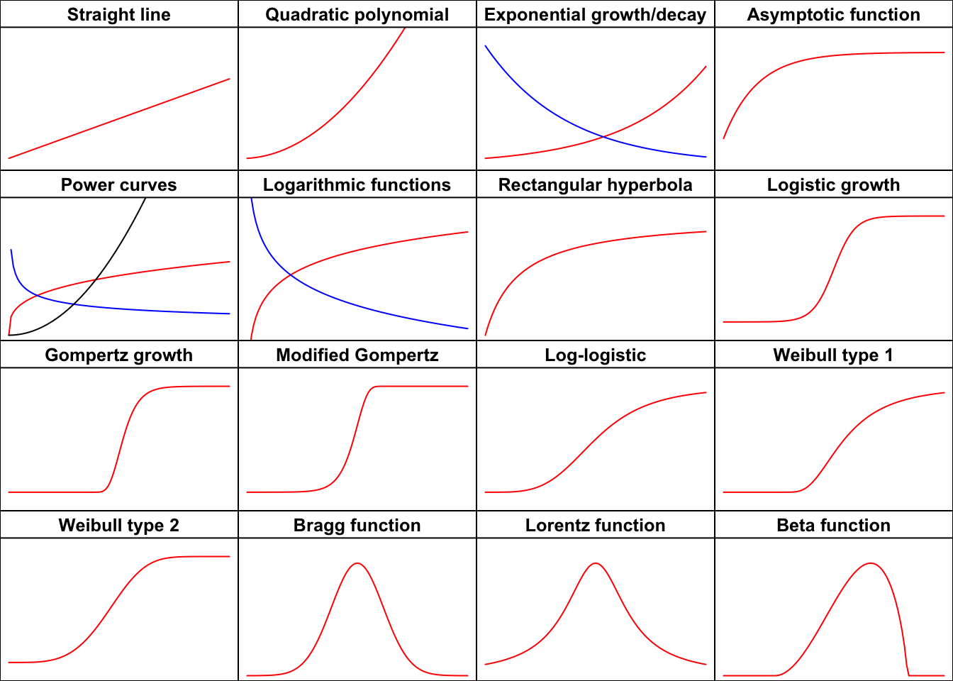
Figure 1: The shapes of the most important functions
Polynomials
Polynomials are a group on their own, as they are characterized by very flexible shapes, which can be used to describe several different biological processes. They are simple and, although they may be curvilinear, they are always linear in the parameters and can be fitted by using least squares methods. One disadvantage is that they cannot describe asymptotic processes, which are very common in biology. Furthermore, polynomials are prone to overfitting, as we may be tempted to add terms to improve the fit, with little care for biological realism.
Nowadays, thanks to the wide availability of nonlinear regression algorithms, the use of polynomials has sensibly decreased; linear or quadratic polynomials are mainly used when we want to approximate the observed response within a narrow range of a quantitative predictor. On the other hand, higher order polynomials are very rarely seen, in practice.
Straight line function
Among the polynomials, we should cite the straight line. Obviously, this is not a curve, although it deserves to be mentioned here. The equation is:
\[Y = b_0 + b_1 \, X \quad \quad \quad (1)\]
where \(b_0\) is the value of \(Y\) when \(X = 0\), \(b_1\) is the slope, i.e. the increase/decrease in \(Y\) for a unit-increase in \(X\). The Y increases as X increases when \(b_1 > 0\), otherwise it decreases. Straight lines are the most common functions for regression and they are most often used to approximate biological phenomena within a small range for the predictor.
Quadratic polynomial function
The quadratic polynomial is:
\[Y = b_0 + b_1\, X + b_2 \, X^2 \quad \quad \quad (2)\]
where \(b_0\) is the value of \(Y\) when \(X = 0\), while \(b_1\) and \(b_2\), taken separately, lack a clear biological meaning. However, it is interesting to consider the first derivative, which measures the rate at which the value \(Y\) changes with respect to the change of \(X\). Calculating a derivative may be tricky for biologists; however, we can make use of the available facilities in R, represented by the D() function, which requires an expression as the argument:
D(expression(a + b*X + c*X^2), "X")
## b + c * (2 * X)
We see that the first derivative is not constant, but it changes according to the level of \(X\). The stationary point, i.e. the point at which the derivative is zero, is \(X_m = - b_1 / 2 b_2\); this point is a maximum when \(b_2 > 0\), otherwise it is a minimum.
The maximum/minimum value is:
\[Y_m = \frac{4\,b_0\,b_2 - b_1^2}{4\,b_2}\]
Polynomial fitting in R
In R, polynomials are fitted by using ‘lm()’. In a couple of cases, I found myself in the need of fitting a polynomial by using nonlinear regression with ‘nls()’ o ‘drm()’. I know, this is not efficient…, but some methods for ‘drc’ objects are rather handy. For these unusual cases, we can use the NLS.linear(), NLS.poly2(), DRC.linear() and DRC.poly2() self-starting functions, as available in the ‘aomisc’ package. An example of usage is given below: in this case, the polynomial has been used to describe a concave increasing trend.
X <- seq(5, 50, 5)
Y <- c(12.6, 74.1, 157.6, 225.5, 303.4, 462.8,
       669.9, 805.3, 964.2, 1169)

# nls fit
model <- nls(Y ~ NLS.poly2(X, a, b, c))

#drc fit
model <- drm(Y ~ X, fct = DRC.poly2())
summary(model)
##
## Model fitted: Second Order Polynomial (3 parms)
##
## Parameter estimates:
##
##                 Estimate Std. Error t-value  p-value
## a:(Intercept) -23.515000  31.175143 -0.7543  0.47528
## b:(Intercept)   5.466470   2.604011  2.0993  0.07395 .
## c:(Intercept)   0.371561   0.046141  8.0527 8.74e-05 ***
## ---
## Signif. codes:  0 '***' 0.001 '**' 0.01 '*' 0.05 '.' 0.1 ' ' 1
##
## Residual standard error:
##
##  26.50605 (7 degrees of freedom)
 r
plot(model, log = "", main = "2nd order polynomial")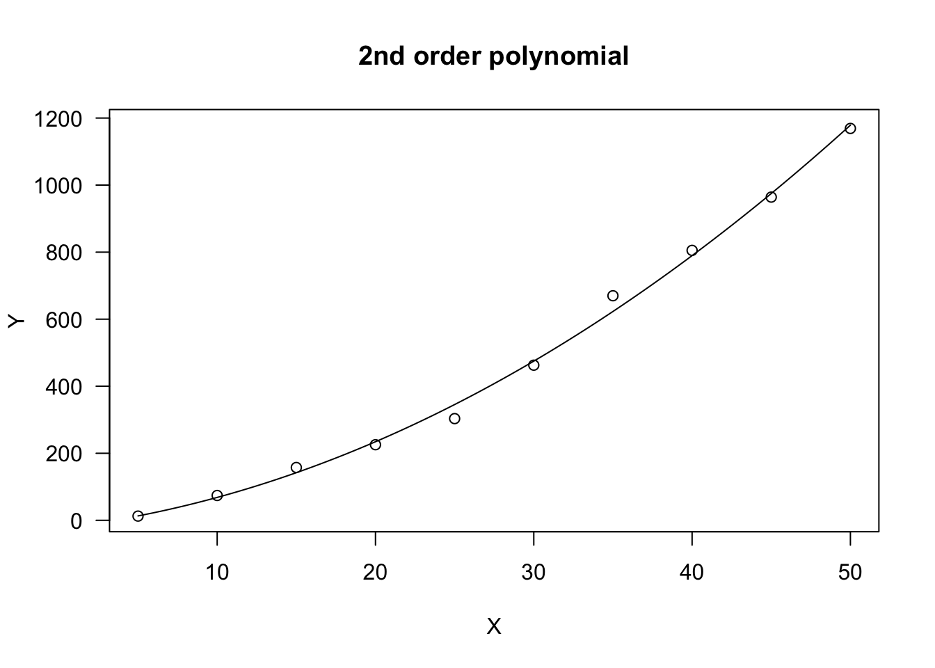
Concave/Convex curves
Exponential function
The exponential function describes an increasing/decreasing trend, with constant relative rate. The most common equation is:
\[ Y = a e^{k X} \quad \quad \quad (3) \]
Two additional and equivalent parameterisations are:
\[ Y = a b^X = e^{d + k X} \quad \quad \quad (4)\]
The Equations 3 and the two equations 4 are equivalent, as proved by setting \(b = e^k\) e \(a = e^d\):
\[a b^X = a (e^k)^{X} = a e^{kX}\]
and:
\[a e^{kX} = e^d \cdot e^{kX} = e^{d + kX}\]
The meaning of \(a\) is clear: this is the value of \(Y\) when \(X = 0\). In order to understand the meaning of \(k\), we can calculate the first derivative of the exponential function:
D(expression(a * exp(k * X)), "X")
## a * (exp(k * X) * k)
From there, we see that the ratio of increase/decrease of \(Y\) is:
\[ \frac{dY}{dX} = k \, a \, e^{k \, X} = k \, Y\]
That is, the relative ratio of increase/decrease is constant and equal to \(k\):
\[ \frac{dY}{dX} \frac{1}{Y} = k\]
\(Y\) increases as \(X\) increases if \(k > 0\) (exponential growth), while it decreases when \(k < 0\) (exponential decay). This curve is used to describe the growth of populations in non-limiting environmental conditions, or to describe the degradation of xenobiotics in the environment (first-order degradation kinetic).
Another slightly different parameterisation exists, which is common in bioassay work and it is mainly used as an exponential decay model:
\[ Y = d \exp(-x/e) \quad \quad \quad (5)\]
where \(d\) is the same as \(a\) in the model above and \(e = - 1/k\). For all the aforementioned exponential decay equations \(Y \rightarrow 0\) as \(X \rightarrow \infty\). In the above curve, a lower asymptote \(c \neq 0\) can also be included, for those situations where the phenomenon under study does not approach 0 when the independent variable approaches infinity:
\[ Y = c + (d -c) \exp(-x/e) \quad \quad \quad (6)\]
The exponential function is nonlinear in \(k\) and needs to be fitted by using ‘nls()’ or ‘drm()’. Several self-starting functions are available: in the package aomisc you can find NLS.expoGrowth(), NLS.expoDecay(), DRC.expoGrowth() and DRC.expoDecay(), which can be used to fit the Equation 3, respectively with ‘nls()’ and ‘drm()’. The ‘drc’ package also contains the functions EXD.2() and EXD.3(), which can be used to fit, respectively, the Equations 5 and 6. Examples of usage are given below.
data(degradation)

# nls fit
model <- nls(Conc ~ NLS.expoDecay(Time, a, k),
             data = degradation)

# drm fit
model <- drm(Conc ~ Time, fct = DRC.expoDecay(),
             data = degradation)
summary(model)
##
## Model fitted: Exponential Decay Model (2 parms)
##
## Parameter estimates:
##
##                  Estimate Std. Error t-value   p-value
## C0:(Intercept) 99.6349312  1.4646680  68.026 < 2.2e-16 ***
## k:(Intercept)   0.0670391  0.0019089  35.120 < 2.2e-16 ***
## ---
## Signif. codes:  0 '***' 0.001 '**' 0.01 '*' 0.05 '.' 0.1 ' ' 1
##
## Residual standard error:
##
##  2.621386 (22 degrees of freedom)
 r
plot(model, log = "", main = "Exponential decay", ylim = c(0, 110))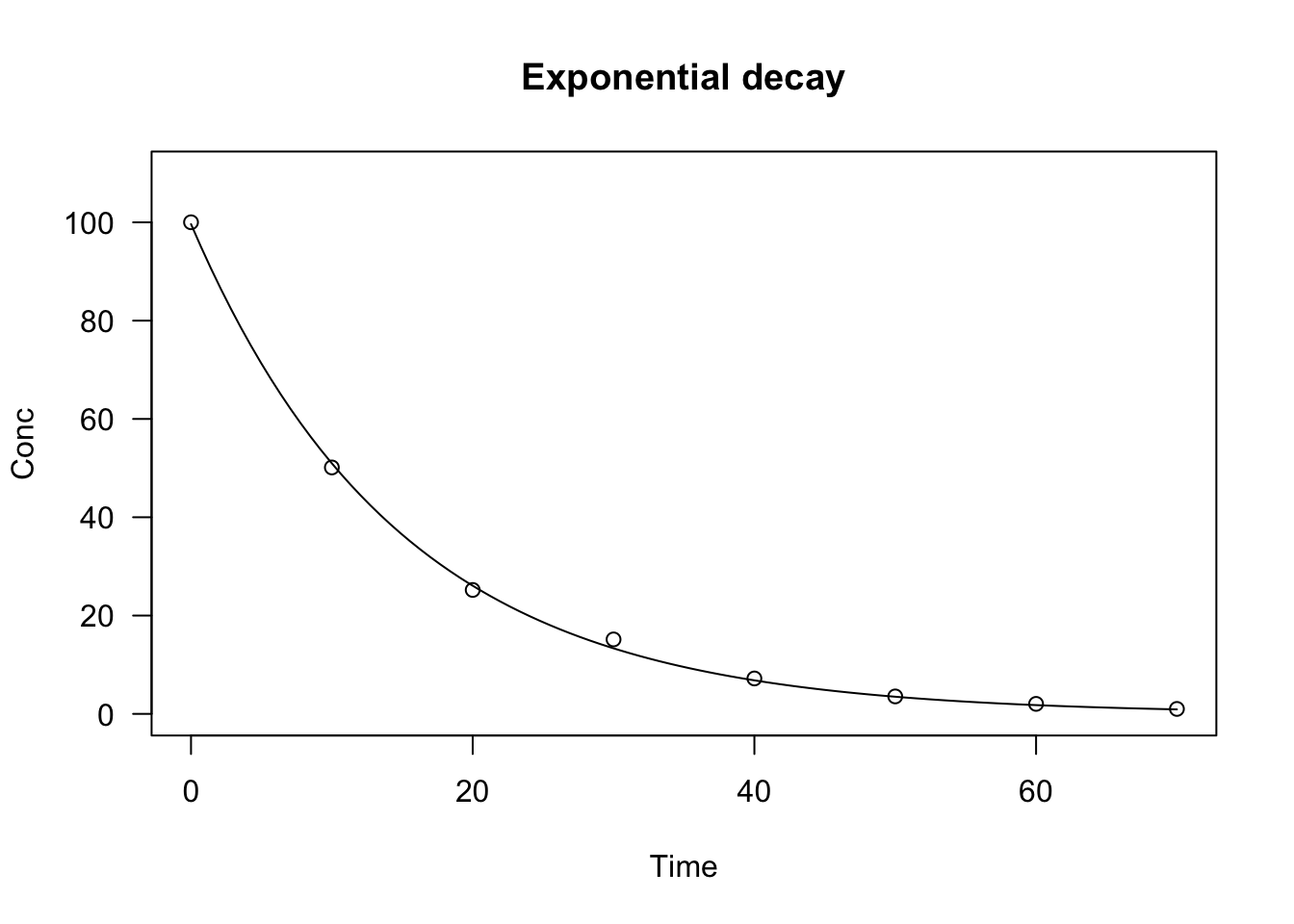
Asymptotic function
The asymptotic function can be used to model the growth of a population/individual, where \(Y\) approaches an horizontal asymptote as \(X\) tends to infinity. This function is used in several different parameterisations and it is also known as the monomolecular growth function, the Mitscherlich law or the von Bertalanffy law. Due to its biological meaning, the most widespread parameterisation is:
\[Y = a - (a - b) \, \exp (- c X) \quad \quad \quad (7)\]
where \(a\) is the maximum attainable value for \(Y\) (plateau), \(b\) is the initial \(Y\) value (at \(X = 0\)) and \(c\) is proportional to the relative rate of increase for \(Y\) when \(X\) increases. Indeed, we can see that the first derivative is:
D(expression(a - (a - b) * exp (- c * X)), "X")
## (a - b) * (exp(-c * X) * c)
that is, the absolute ratio of increase of \(Y\) at a given \(X\) is not constant, but depends on the attained value of \(Y\):
\[ \frac{dY}{dX} = c \, (a - Y)\]
If we consider the relative rate of increase of \(Y\), we see that:
\[\frac{dY}{dX} \frac{1}{Y} = c \, \frac{(a - Y)}{Y}\]
It means that the relative rate of increase of \(Y\) is maximum at the beginning and approaches 0 when \(Y\) approaches the plateau \(a\).
In order to fit the asymptotic function, the ‘aomisc’ package contains the self-starting routines NLS.asymReg() and DRC.asymReg(), which can be used, respectively, with ‘nls()’ and ‘drm()’. The ‘drc’ package contains the function AR.3(), that is a similar parameterisation where \(c\) is replaced by \(e = 1/c\). The ‘nlme’ package also contains an alternative parameterisation, named SSasymp(), where \(c\) is replaced by \(\phi_3 = \log(c)\).
Let’s see an example.
X <- c(1, 3, 5, 7, 9, 11, 13, 20)
Y <- c(8.22, 14.0, 17.2, 16.9, 19.2, 19.6, 19.4, 19.6)

# nls fit
model <- nls(Y ~ NLS.asymReg(X, init, m, plateau) )

# drm fit
model <- drm(Y ~ X, fct = DRC.asymReg())
plot(model, log="", main = "Asymptotic regression",
     ylim = c(0,25), xlim = c(0,20))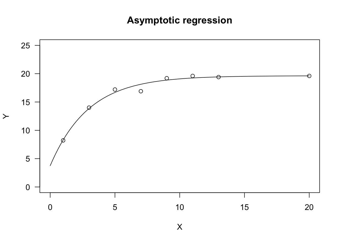
If we take the asymptotic function and set \(b = 0\), we get the negative exponential function:
\[Y = a [1 - \exp (- c X) ] \quad \quad \quad (8)\]
This function shows a similar shape as the asymptotic function, but \(Y\) is 0 when \(X\) is 0 (the curve passes through the origin). It is often used to model the absorbed Photosintetically Active Radiation (\(Y = PAR_a\)) as a function of Leaf Area Index (X = LAI). In this case, \(a\) represents the incident PAR (\(a = PAR_i\)), and \(c\) represents the extinction coefficient.
In order to fit the Equation 8, we can use the self-starters NLS.negExp() with ‘nls()’ and DRC.negExp() with ‘drm()’; both self-starters are available within the ‘aomisc’ package. The ‘drc’ package contains the function AR.2(), where \(c\) is replaced by \(e = 1/c\). The ‘nlme’ package also contains an alternative parameterisation, named SSasympOrig(), where \(c\) is replaced by \(\phi_3 = \log(c)\).
Power function
The power function is also known as Freundlich function or allometric function and the most common parameterisation is:
\[Y = a \, X^b \quad \quad \quad (9)\]
This curve is perfectly equivalent to an exponential curve on the logarithm of \(X\). Indeed:
\[a\,X^b = a\, e^{\log( X^b )} = a\,e^{b \, \log(x)}\]
This curve does not have an asymptote for \(X \rightarrow \infty\). The slope (first derivative) of the curve is:
D(expression(a * X^b), "X")
## a * (X^(b - 1) * b)
We see that both parameters relate to the ‘slope’ of the curve and \(b\) dictates its shape. If \(0 < b < 1\), the response \(Y\) increases as \(X\) increases and the curve is convex up. If \(b < 0\), the curve is concave up and \(Y\) decreases as \(X\) increases. Otherwise, if \(b > 1\), the curve is concave up and \(Y\) increases as \(X\) increases. The three curve types are shown in Figure 1, above.
The power function (Freundlich equation) is often used in agricultural chemistry, e.g. to model the sorption of xenobiotics in soil. It is also used to model the number of plant species as a function of sampling area (Muller-Dumbois method). The following example uses the DRC.powerCurve() and NLS.powerCurve() self starters in the ‘aomisc’ package to fit a species-area curve.
data(speciesArea)

#nls fit
model <- nls(numSpecies ~ NLS.powerCurve(Area, a, b),
             data = speciesArea)

# drm fit
model <- drm(numSpecies ~ Area, fct = DRC.powerCurve(),
             data = speciesArea)
summary(model)
##
## Model fitted: Power curve (Freundlich equation) (2 parms)
##
## Parameter estimates:
##
##               Estimate Std. Error t-value   p-value
## a:(Intercept) 4.348404   0.337197  12.896 3.917e-06 ***
## b:(Intercept) 0.329770   0.016723  19.719 2.155e-07 ***
## ---
## Signif. codes:  0 '***' 0.001 '**' 0.01 '*' 0.05 '.' 0.1 ' ' 1
##
## Residual standard error:
##
##  0.9588598 (7 degrees of freedom)
Logarithmic function
This is indeed a linear model on log-transformed \(X\):
\[y = a + b \, \log(X) \quad \quad \quad (10)\]
Due to the logarithmic function, it must be \(X > 0\). The parameter \(b\) dictates the shape: if \(b > 0\), the curve is convex up and \(Y\) increases as \(X\) increases. If \(b < 0\), the curve is concave up and \(Y\) decreases as \(X\) increases, as shown in Figure 1 above.
The logarithmic equation can be fit by using ‘lm()’. If necessary, it can also be fit by using ‘nls()’ and ‘drm()’: the self-starting functions NLS.logCurve() and DRC.logCurve() are available within the ‘aomisc’ package. We show an example of their usage in the box below.
X <- c(1,2,4,5,7,12)
Y <- c(1.97, 2.32, 2.67, 2.71, 2.86, 3.09)

# lm fit
model <- lm(Y ~ log(X) )

# nls fit
model <- nls(Y ~ NLS.logCurve(X, a, b) )

# drm fit
model <- drm(Y ~ X, fct = DRC.logCurve() )
Rectangular hyperbola
This function is also known as the Michaelis-Menten function and it is often parameterised as:
\[Y = \frac{a \, X} {b + X} \quad \quad \quad (11)\]
The curve is convex up and \(Y\) increases as \(X\) increases, up to a plateau level. The parameter \(a\) represents the higher asymptote (for \(X \rightarrow \infty\)), while \(b\) is the X value giving a response equal to \(a/2\). Indeed, it is easily shown that:
\[\frac{a}{2} = \frac{a\,X_{50} } {b + X_{50} } \]
which leads to \(b = x_{50}\).
The slope (first derivative) is:
D(expression( (a*X) / (b + X) ), "X")
## a/(b + X) - (a * X)/(b + X)^2
From there, we can see that the initial slope (at \(X = 0\)) is $i = a/b $. The equation 11 is not defined for \(X = b\) and it makes no biological sense for \(X < b\).
An alternative parameterisation is obtained considering that:
\[Y = \frac{a \, X} {b + X} = \frac{a}{ \frac{b}{X} + \frac{X}{X}} = \frac{a}{1 + \frac{b}{X}} \quad \quad \quad (12)\]
This parameterisation is sometimes used in bioassays and it is parameterised with \(d = a\) and \(e = b\). From a strict mathematical point of view, the equation 12 is not defined for \(X = 0\), although it approaches 0 when \(X \rightarrow 0\).
The Michaelis-Menten function is used in pesticide chemistry, enzyme kinetics and in weed competition studies, to model yield losses as a function of weed density. In R, this model can be fit by using ‘nls()’ and the self-starting functions SSmicmen(), within the package ‘nlme’. If you prefer a ‘drm()’ fit, you can use the MM.2() function in the ‘drc’ package, which uses the parameterisation in Equation 12.
X <- c(0, 5, 7, 22, 28, 39, 46, 200)
Y <- c(12.74, 13.66, 14.11, 14.43, 14.78, 14.86, 14.78, 14.91)

#drm fit
model <- drm(Y ~ X, fct = MM.2())
summary(model)
##
## Model fitted: Michaelis-Menten (2 parms)
##
## Parameter estimates:
##
##               Estimate Std. Error t-value  p-value
## d:(Intercept) 14.93974    2.86695  5.2110 0.001993 **
## e:(Intercept)  0.45439    2.24339  0.2025 0.846183
## ---
## Signif. codes:  0 '***' 0.001 '**' 0.01 '*' 0.05 '.' 0.1 ' ' 1
##
## Residual standard error:
##
##  5.202137 (6 degrees of freedom)
 r
plot(model, log = "", main = "Michaelis-Menten function",
     ylim = c(12, 15))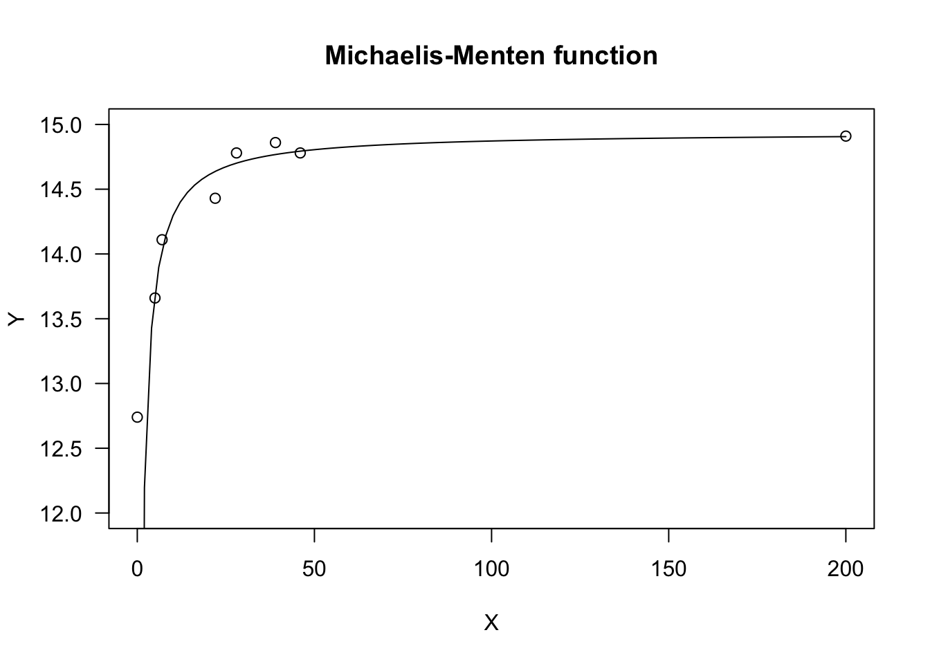
Sigmoidal curves
Sigmoidal curves are S-shaped and they may be increasing, decreasing, symmetric or non-symmetric around the inflection point. They are parameterised in countless ways, which may often be confusing. I will show some widespread parameterisations, that are very useful for bioassays or growth studies. All curves can be turned from increasing to decreasing (and vice-versa) by reversing the sign of the \(b\) parameter.
Logistic function
The logistic curve derives from the cumulative logistic distribution function; the curve is symmetric around the inflection point and it may be parameterised as:
\[Y = c + \frac{d - c}{1 + exp(- b (X - e))} \quad \quad \quad (13)\]
where \(d\) is the higher asymptote, \(c\) is the lower asymptote, \(e\) is \(X\) value at the inflection point, while \(b\) is the slope at the inflection point. As the curve is symmetric, \(e\) represents also the \(X\) value producing a response half-way between \(d\) and \(c\) (usually known as the ED50, in biological assay). The parameter \(b\) can be positive or negative and, consequently, \(Y\) may increase or decrease as \(X\) increases.
The above function is known as the four-parameter logistic. If necessary, constraints can be put on parameter values, i.e. \(c\) can be constrained to 0 (three-parameter logistic) and, additionally, \(d\) can be constrained to 1 (two-parameter logistic).
In the ‘aomisc’ package, the three logistic curves (four-, three- and two-parameters) are available as NLS.L4(), NLS.L3() and NLS.L2(), respectively. With ‘drm()’, we can use the self-starting functions L.4() and L.3() in the package ‘drc’, while the L.2() function for the two-parameter logistic has been included in the ‘aomisc’ package. The only difference between the self-starters for ‘drm()’ and the self-starters for ‘nls()’ is that, in the former, the sign for the \(b\) parameter is reversed, i.e. it is negative for increasing curves and positive for decreasing curves.
The four- and three-parameter logistic curves can also be fit with ‘nls()’, respectively with the self-starting functions SSfpl() and SSlogis(), in the ‘nlme’ package. In these functions, \(b\) is replaced by \(scal = -1/b\).
In the box below, I show an example, regarding the growth of a sugar-beet crop.
data(beetGrowth)

# nls fit
model <- nls(weightInf ~ NLS.L3(DAE, b, d, e), data = beetGrowth)
model.2 <- nls(weightInf ~ NLS.L4(DAE, b, c, d, e), data = beetGrowth)
model.3 <- nls(weightInf/max(weightInf) ~ NLS.L2(DAE, b, e), data = beetGrowth)

# drm fit
model <- drm(weightInf ~ DAE, fct = L.3(), data = beetGrowth)
model.2 <- drm(weightInf ~ DAE, fct = L.4(), data = beetGrowth)
model.3 <- drm(weightInf/max(weightInf) ~ DAE, fct = L.2(), data = beetGrowth)
summary(model)
##
## Model fitted: Logistic (ED50 as parameter) with lower limit fixed at 0 (3 parms)
##
## Parameter estimates:
##
##                Estimate Std. Error t-value   p-value
## b:(Intercept) -0.118771   0.018319 -6.4835 1.032e-05 ***
## d:(Intercept) 25.118357   1.279417 19.6327 4.127e-12 ***
## e:(Intercept) 58.029764   1.834414 31.6340 3.786e-15 ***
## ---
## Signif. codes:  0 '***' 0.001 '**' 0.01 '*' 0.05 '.' 0.1 ' ' 1
##
## Residual standard error:
##
##  2.219389 (15 degrees of freedom)
 r
plot(model, log="", main = "Logistic function")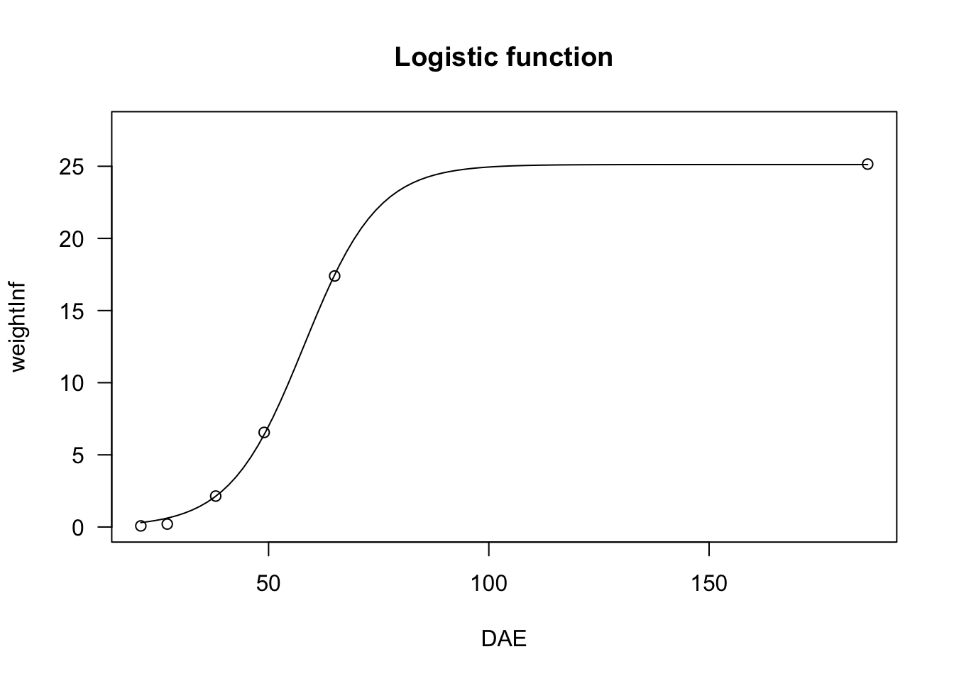
Gompertz function
The Gompertz curve is parameterised in very many ways. I tend to prefer a parameterisation that resembles the one used for the logistic function:
\[ Y = c + (d - c) \exp \left\{- \exp \left[ - b \, (X - e) \right] \right\} \quad \quad \quad (14)\]
The difference between the logistic and Gompertz functions is that this latter is not symmetric around the inflection point: it shows a longer lag at the beginning, but raises steadily afterwards. The parameters have the same meaning as those in the logistic function, apart from the fact that \(e\), i.e. the abscissa of the inflection point, does not give a response half-way between \(c\) and \(d\). As for the logistic, we can have four-, three- and two-parameter Gompertz functions, which can be used to describe plant growth or several other biological processes.
In R, the Gompertz equation can be fit by using ‘drm()’ and, respectively the G.4(), G.3() and G.2() self-starters. With ‘nls’, the ‘aomisc’ package contains the corresponding functions NLS.G4(), NLS.G3() and NLS.G2(). As for the logistic, the only difference between the self starters for ‘drm()’ and the self starters for ‘nls()’ is that, in the former, the sign for the \(b\) parameter is reversed, i.e. it is negative for increasing curves and positive for decreasing curves.
The three-parameter Gompertz can also be fit with ‘nls()’, by using the SSGompertz() self-starter in the ‘nlme’ package, although this is a different parameterisation.
# nls fit
model <- nls(weightFree ~ NLS.G3(DAE, b, d, e), data = beetGrowth)
model.2 <- nls(weightFree ~ NLS.G4(DAE, b, c, d, e), data = beetGrowth)
model.3 <- nls(weightFree/max(weightFree) ~ NLS.G2(DAE, b, e), data = beetGrowth)

# drm fit
model <- drm(weightFree ~ DAE, fct = G.3(), data = beetGrowth)
model.2 <- drm(weightFree ~ DAE, fct = G.4(), data = beetGrowth)
model.3 <- drm(weightFree/max(weightFree) ~ DAE, fct = G.2(), data = beetGrowth)
summary(model)
##
## Model fitted: Gompertz with lower limit at 0 (3 parms)
##
## Parameter estimates:
##
##                Estimate Std. Error t-value   p-value
## b:(Intercept) -0.122255   0.029938 -4.0836 0.0009783 ***
## d:(Intercept) 35.078529   1.668665 21.0219 1.531e-12 ***
## e:(Intercept) 49.008075   1.165191 42.0601 < 2.2e-16 ***
## ---
## Signif. codes:  0 '***' 0.001 '**' 0.01 '*' 0.05 '.' 0.1 ' ' 1
##
## Residual standard error:
##
##  2.995873 (15 degrees of freedom)
 r
plot(model, log="", main = "Gompertz function")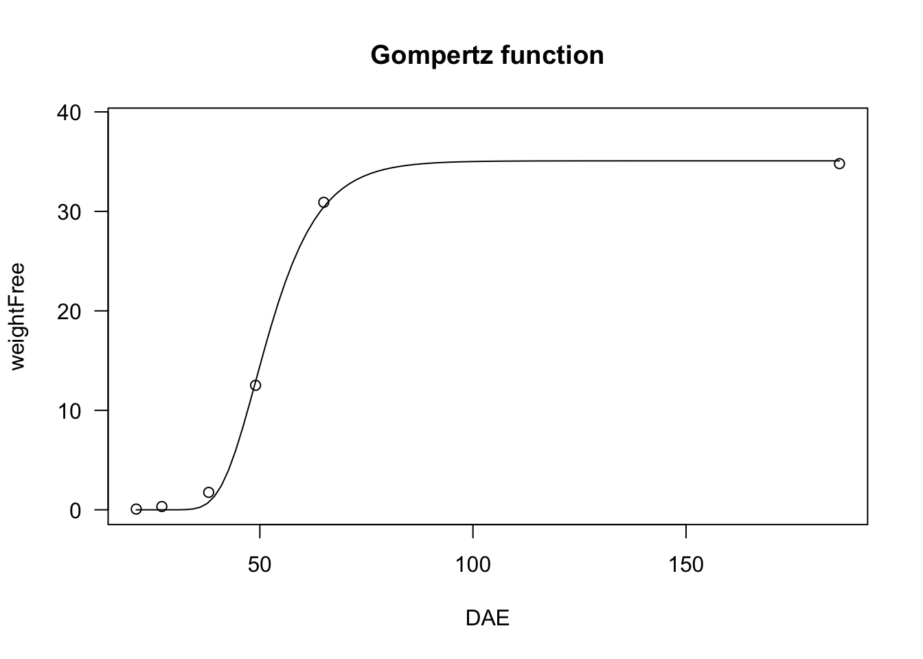
Modified Gompertz function
We have seen that the logistic curve is symmetric around the inflection point, while the Gompertz shows a longer lag at the beginning and raises steadily afterwards. We can describe a different pattern by modifying the Gompertz function as follows:
\[ Y = c + (d - c) \left\{ 1 - \exp \left\{- \exp \left[ b \, (X - e) \right] \right\} \right\} \quad \quad \quad (15)\]
The resulting curve increases steadily at the beginning, but slows down later on. Also for this function, we can put constraints on \(d = 1\) and/or \(c = 0\), so that we have four-parameter, three-parameter and two-parameter modified Gompertz equations; these models can be fit by using ‘nls()’ and the self starters NLS.E4(), NLS.E3() and NLS.E2() in the ‘aomisc’ package. Likewise, the modified Gompertz equations can be fit with ‘drm()’ and the self starters E.4(), E.3() and E.2(), also available in the ‘aomisc’ package
# nls fit
model <- nls(weightInf ~ NLS.E3(DAE, b, d, e), data = beetGrowth)
model.2 <- nls(weightFree ~ NLS.E4(DAE, b, c, d, e), data = beetGrowth)
model.3 <- nls(I(weightFree/max(weightFree)) ~ NLS.E2(DAE, b, e), data = beetGrowth)


# drm fit
model <- drm(weightInf ~ DAE, fct = E.3(), data = beetGrowth)
model.2 <- drm(weightFree ~ DAE, fct = E.4(), data = beetGrowth)
model.3 <- drm(weightFree/max(weightFree) ~ DAE, fct = E.2(), data = beetGrowth)
summary(model)
##
## Model fitted: Modified Gompertz equation (3 parameters) (3 parms)
##
## Parameter estimates:
##
##                Estimate Std. Error t-value   p-value
## b:(Intercept)  0.092508   0.013231  6.9917 4.340e-06 ***
## d:(Intercept) 25.107004   1.304379 19.2482 5.493e-12 ***
## e:(Intercept) 63.004111   1.747087 36.0624 4.945e-16 ***
## ---
## Signif. codes:  0 '***' 0.001 '**' 0.01 '*' 0.05 '.' 0.1 ' ' 1
##
## Residual standard error:
##
##  2.253878 (15 degrees of freedom)
 r
plot(model, log="", main = "Modified Gompertz")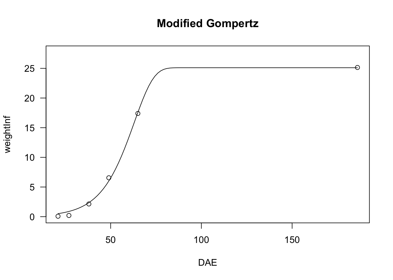
Log-logistic function
The log-logistic curve is symmetric on the logarithm of \(X\) (a log-normal curve would be practically equivalent, but it is used far less often). For example, in biologic assays (but also in germination assays), the log-logistic curve is defined as follows:
\[Y = c + \frac{d - c}{1 + \exp \left\{ - b \left[ \log(X) - \log(e) \right] \right\} } \quad \quad \quad (16)\]
The parameters have the same meaning as the logistic equation given above. In particular, \(e\) represents the X-level which gives a response half-way between \(c\) and \(d\) (ED50). It is easy to see that the above equation is equivalent to:
\[Y = c + \frac{d - c}{1 + \left( \frac{X}{e} \right)^{-b}}\]
Log-logistic functions are used for crop growth, seed germination and bioassay work and they can have the same constraints as the logistic function (four- three- and two-parameter log-logistic). They can be fit by ‘drm()’ and the self starters LL.4() (four-parameter log-logistic), LL.3() (three-parameter log-logistic, with \(c = 0\)) and LL.2() (two-parameter log-logistic, with \(d = 1\) and \(c = 0\)), as available in the ‘drc’ package. With respect to Equation 16, in these self-starters the sign for \(b\) is reversed, i.e. it is negative for the increasing log-logistic curve and positive for the decreasing curve. In the package ‘aomisc’, the corresponding self starters for ‘nls()’ are NLS.LL4(), NLS.LL3() and NLS.LL2(), which are all derived from Equation 15 (i.e. the sign of \(b\) is positive for increasing curves and negative for decreasing curves).
We show an example of a log-logistic fit, relating to a bioassay with Brassica rapa treated at increasing dosages of an herbicide.
data(brassica)

model <- nls(FW ~ NLS.LL4(Dose, b, c, d, e), data = brassica)
model <- nls(FW ~ NLS.LL3(Dose, b, d, e), data = brassica)
model <- nls(FW/max(FW) ~ NLS.LL2(Dose, b, e), data = brassica)

model <- drm(FW ~ Dose, fct = LL.4(), data = brassica)
summary(model)
##
## Model fitted: Log-logistic (ED50 as parameter) (4 parms)
##
## Parameter estimates:
##
##               Estimate Std. Error t-value   p-value
## b:(Intercept)  1.45113    0.24113  6.0181 1.743e-06 ***
## c:(Intercept)  0.34948    0.18580  1.8810   0.07041 .
## d:(Intercept)  4.53636    0.20514 22.1140 < 2.2e-16 ***
## e:(Intercept)  2.46557    0.35111  7.0221 1.228e-07 ***
## ---
## Signif. codes:  0 '***' 0.001 '**' 0.01 '*' 0.05 '.' 0.1 ' ' 1
##
## Residual standard error:
##
##  0.4067837 (28 degrees of freedom)
 r
plot(model, ylim = c(0,6), main = "Log-logistic function")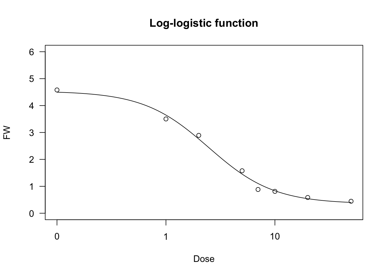
Weibull function (type 1)
The type 1 Weibull function corresponds to the Gompertz, but it is based on the logarithm of \(X\). The equation is as follows:
\[ Y = c + (d - c) \exp \left\{- \exp \left[ - b \, (\log(X) - \log(e)) \right] \right\} \quad \quad \quad (17)\]
The parameters have the same meaning as the other sigmoidal curves given above, apart from the fact that \(e\) is the abscissa of the inflection point, but it is not the ED50.
The four-parameters, three-parameters and two-parameters Weibull functions can be fit by using ‘drm()’ and the self-starters available within the ‘drc’ package, i.e. W1.4(), W1.3() and W1.2(). The ‘aomisc’ package contains the corresponding self-starters NLS.W1.4(), NLS.W1.3() and NLS.W1.2(), which can be used with ‘nls()’.
data(brassica)

model <- nls(FW ~ NLS.W1.4(Dose, b, c, d, e), data = brassica)
model.2 <- nls(FW ~ NLS.W1.3(Dose, b, d, e), data = brassica)
model.3 <- nls(FW/max(FW) ~ NLS.W1.2(Dose, b, e), data = brassica)

model <- drm(FW ~ Dose, fct = W1.4(), data = brassica)
model.2 <- drm(FW ~ Dose, fct = W1.3(), data = brassica)
model.3 <- drm(FW/max(FW) ~ Dose, fct = W1.2(), data = brassica)
summary(model)
##
## Model fitted: Weibull (type 1) (4 parms)
##
## Parameter estimates:
##
##               Estimate Std. Error t-value   p-value
## b:(Intercept)  1.01252    0.15080  6.7143 2.740e-07 ***
## c:(Intercept)  0.50418    0.14199  3.5507  0.001381 **
## d:(Intercept)  4.56137    0.19846 22.9841 < 2.2e-16 ***
## e:(Intercept)  3.55327    0.45039  7.8894 1.359e-08 ***
## ---
## Signif. codes:  0 '***' 0.001 '**' 0.01 '*' 0.05 '.' 0.1 ' ' 1
##
## Residual standard error:
##
##  0.3986775 (28 degrees of freedom)
 r
plot(model, ylim = c(0,6), main = "Weibull type 1")
Weibull function (type 2)
The type 2 Weibull is similar to the type 1 Weibull, but describes a different type of asymmetry, corresponding to the modified Gompertz function above:
\[ Y = c + (d - c) \left\{ 1 - \exp \left\{- \exp \left[ b \, (\log(X) - \log(e)) \right] \right\} \right\} \quad \quad \quad (18)\]
As for fitting, the ‘drc’ package contains the self-starting functions W2.4(), W2.3() and W2.2(), which can be used with ‘drm()’ (be careful: the sign for \(b\) is reversed, with respect to Equation 18). The ‘aomisc’ package contains the corresponding self-starters NLS.W2.4(), NLS.W2.3() and NLS.W2.2(), which can be used with ‘nls()’.
data(brassica)

model <- nls(FW ~ NLS.W2.4(Dose, b, c, d, e), data = brassica)
model.1 <- nls(FW ~ NLS.W2.3(Dose, b, d, e), data = brassica)
model.2 <- nls(FW/max(FW) ~ NLS.W2.2(Dose, b, e), data = brassica)

model <- drm(FW ~ Dose, fct = W2.4(), data = brassica)
summary(model)
##
## Model fitted: Weibull (type 2) (4 parms)
##
## Parameter estimates:
##
##               Estimate Std. Error t-value   p-value
## b:(Intercept) -0.96191    0.17684 -5.4395 8.353e-06 ***
## c:(Intercept)  0.18068    0.25191  0.7173    0.4792
## d:(Intercept)  4.53804    0.21576 21.0328 < 2.2e-16 ***
## e:(Intercept)  1.66342    0.25240  6.5906 3.793e-07 ***
## ---
## Signif. codes:  0 '***' 0.001 '**' 0.01 '*' 0.05 '.' 0.1 ' ' 1
##
## Residual standard error:
##
##  0.4215551 (28 degrees of freedom)
 r
plot(model, ylim = c(0,6), main = "Weibull type 2")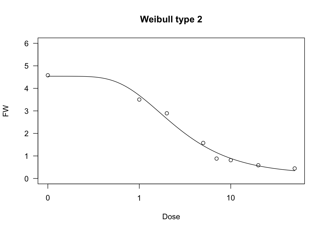
Curves with maxima/minima
It is sometimes necessary to describe phenomena where the \(Y\) variable reaches a maximum value at a certain level of the \(X\) variable, and drops afterwords. For example, growth or germination rates are higher at optimal temperature levels and lower at supra-optimal or sub-optimal temperature levels. Another example relates to bioassays: in some cases, low doses of toxic substances induce a stimulation of growth (hormesis), which needs to be described by an appropriate model. Let’s see some functions which may turn out useful in these circumstances.
Bragg function
This function is connected to the normal (Gaussian) distribution and has a symmetric shape with a maximum equal to \(d\), that is reached when \(X = e\) and two inflection points. In this model, \(b\) relates to the slope at the inflection points; the response \(Y\) approaches 0 when \(X\) approaches \(\pm \infty\):
\[ Y = d \, \exp \left[ - b (X - e)^2 \right] \quad \quad \quad (19)\]
If we would like to have lower asymptotes different from 0, we should add the parameter \(c\), as follows:
\[ Y = c + (d - c) \, \exp \left[ - b (X - e)^2 \right] \quad \quad \quad (20)\]
The two Bragg curves have been used in applications relating to the science of carbon materials. We can fit them with ‘drm()’, by using the self starters DRC.bragg.3() (Equation 19) and DRC.bragg.4 (Equation 20), in the ‘aomisc’ package. With ‘nls()’, you can use the corresponding self-starters NLS.bragg.3() and NLS.bragg.4, also in the ‘aomisc’ package.
X <- c(5, 10, 15, 20, 25, 30, 35, 40, 45, 50)
Y1 <- c(0.1, 2, 5.7, 9.3, 19.7, 28.4, 20.3, 6.6, 1.3, 0.1)
Y2 <- Y1 + 2

# nls fit
mod.nls <- nls(Y1 ~ NLS.bragg.3(X, b, d, e) )
mod.nls2 <- nls(Y2 ~ NLS.bragg.4(X, b, c, d, e) )

# drm fit
mod.drc <- drm(Y1 ~ X, fct = DRC.bragg.3() )
mod.drc2 <- drm(Y2 ~ X, fct = DRC.bragg.4() )
plot(mod.drc, ylim = c(0, 30), log = "")
plot(mod.drc2, add = T, col = "red")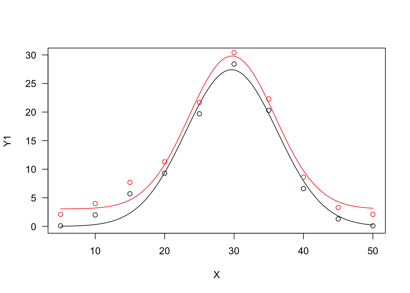
Lorentz function
The Lorentz function is similar to the Bragg function, although it has worse statistical properties (Ratkowsky, 1990). The equation is:
\[ Y = \frac{d} { 1 + b (X - e)^2 } \quad \quad \quad (21)\]
We can also allow for lower asymptotes different from 0, by adding a further parameter:
\[ Y = c + \frac{d - c} { 1 + b (X - e)^2 } \quad \quad \quad (22)\]
The two Lorentz functions can be fit with ‘drm()’, by using the self-starters DRC.lorentz.3() (Equation 21) and DRC.lorentz.4 (Equation 22), in the ‘aomisc’ package. With ‘nls()’, you can use the corresponding self-starters NLS.lorentz.3() and NLS.lorentz.4, also in the ‘aomisc’ package.
X <- c(5, 10, 15, 20, 25, 30, 35, 40, 45, 50)
Y1 <- c(0.1, 2, 5.7, 9.3, 19.7, 28.4, 20.3, 6.6, 1.3, 0.1)
Y2 <- Y1 + 2

# nls fit
mod.nls <- nls(Y1 ~ NLS.lorentz.3(X, b, d, e) )
mod.nls2 <- nls(Y2 ~ NLS.lorentz.4(X, b, c, d, e) )

# drm fit
mod.drc <- drm(Y1 ~ X, fct = DRC.lorentz.3() )
mod.drc2 <- drm(Y2 ~ X, fct = DRC.lorentz.4() )
plot(mod.drc, ylim = c(0, 30), log = "")
plot(mod.drc2, add = T, col = "red")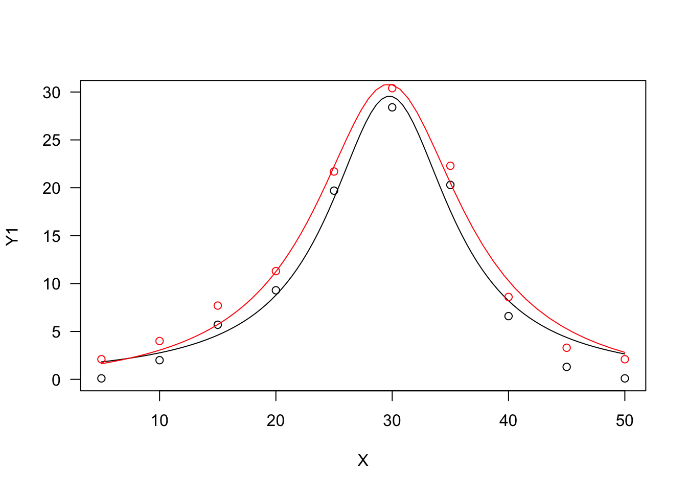
Beta function
The beta function derives from the beta density function and it has been adapted to describe phenomena taking place only within a minimum and a maximum threshold value (threshold model). One typical example is seed germination, where the germination rate (GR, i.e. the inverse of germination time) is 0 below the base temperature level and above the cutoff temperature level. Between these two extremes, the GR increases with temperature up to a maximum level, that is reached at the optimal temperature level.
The equation is:
\[ Y = d \,\left\{ \left( \frac{X - X_b}{X_o - X_b} \right) \left( \frac{X_c - X}{X_c - X_o} \right) ^ {\frac{X_c - X_o}{X_o - X_b}} \right\}^b \quad \quad \quad (23)\]
where \(d\) is the maximum level for the expected response \(Y\), \(X_b\) and \(X_c\) are, respectively, the minumum and maximum threshold levels, \(X_o\) is the abscissa at the maximum expected response level and \(b\) is a shape parameter. The above function is only defined for \(X_b < X < X_c\) and it returns 0 elsewhere.
In R, the beta function can be fitted either with ‘drm()’ and the self-starter DRC.beta(), or with ‘nls()’ and the self-starter NLS.beta(). Both the self-starters are available within the ‘aomisc’ package.
X <- c(1, 5, 10, 15, 20, 25, 30, 35, 40, 45, 50)
Y <- c(0, 0, 0, 7.7, 12.3, 19.7, 22.4, 20.3, 6.6, 0, 0)

model <- nls(Y ~ NLS.beta(X, b, d, Xb, Xo, Xc))
model <- drm(Y ~ X, fct = DRC.beta())
summary(model)
##
## Model fitted: Beta function
##
## Parameter estimates:
##
##                Estimate Std. Error  t-value   p-value
## b:(Intercept)   1.29834    0.26171   4.9609 0.0025498 **
## d:(Intercept)  22.30117    0.53645  41.5715 1.296e-08 ***
## Xb:(Intercept)  9.41770    1.15826   8.1309 0.0001859 ***
## Xo:(Intercept) 31.14068    0.58044  53.6504 2.815e-09 ***
## Xc:(Intercept) 40.47294    0.33000 122.6455 1.981e-11 ***
## ---
## Signif. codes:  0 '***' 0.001 '**' 0.01 '*' 0.05 '.' 0.1 ' ' 1
##
## Residual standard error:
##
##  0.7251948 (6 degrees of freedom)
 r
plot(model, log="", main = "Beta function")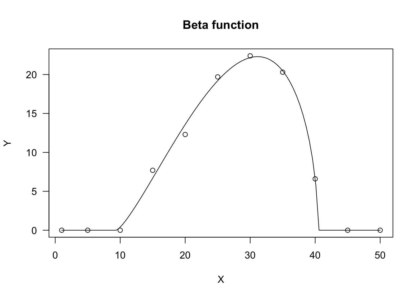
Here we are; I have discussed more than 20 models, which are commonly used for nonlinear regression. These models can be found in several different parameterisations and flavours; they can also be modified and combined to suit the needs of several disciplines in biology, chemistry and so on. However, this will require another post.
Thanks for reading
Andrea Onofri
Department of Agricultural, Food and Environmental Sciences
University of Perugia (Italy)
Borgo XX Giugno 74
I-06121 - PERUGIA
Further readings
- Miguez, F., Archontoulis, S., Dokoohaki, H., Glaz, B., Yeater, K.M., 2018. Chapter 15: Nonlinear Regression Models and Applications, in: ACSESS Publications. American Society of Agronomy, Crop Science Society of America, and Soil Science Society of America, Inc.
- Ratkowsky, D.A., 1990. Handbook of nonlinear regression models. Marcel Dekker Inc., New York, USA.
- Ritz, C., Jensen, S. M., Gerhard, D., Streibig, J. C.
- Dose-Response Analysis Using R. CRC Press