This is a follow-up post. If you are interested in other posts of this series, please go to: https://www.statforbiology.com/tags/drcte/. All these posts expand on a manuscript that we have recently published in the Journal ‘Weed Science’; please follow this link to the paper. In order to work throughout this post, you need to install the ‘drcte’ and ‘drcSeedGerm’ packages, by using the code provided in this page.
Quantiles from time-to-event models
We have previously shown that time-to-event models (e.g., germination or emergence models) can be used to describe the time course of germinations/emergences for a seed lot (this post) or for several seed lots, submitted to different experimental treatments (this post). We have seen that fitted models can be used to extract information of biological relevance (this post).
A time-to-event model is, indeed, a cumulative probability function for germination time and, therefore, we might be interested in finding the quantiles. But, what are the ‘quantiles’? It is a set of ‘cut-points’ that divide the distribution of event-times into a set of \(q\) intervals with equal probability. For example the 100-quantiles, also named as the percentiles, divide the distribution of event-times into \(q = 100\) groups. Some of these cut-off points may be particularly relevant: for example the 50-th percentile corresponds to the time required to reach 50% germination (T50) and it is regarded as a good measure of germination velocity. Other common percentiles are the T10, or the T30, which are used to express the germination velocity for the quickest seeds in the lot.
Extracting some relevant percentiles from the time-to-event curve is regarded as an important task, to sintetically describe the germination/emergence velocity of seed populations. To this aim, we have included the quantile() method in the drcte package, that addresses most of the peculiarities of seed germination/emergence data. In this post, we will show the usage of this function.
Peculiarities of seed science data
I know that you are looking forward to getting the quantiles for your time-to-event curve. Please, hang on for a while… we need to become aware of a couple of issues, that are specific to germination/emergence data and are not covered in literature for other types of time-to-event data (e.g., survival data).
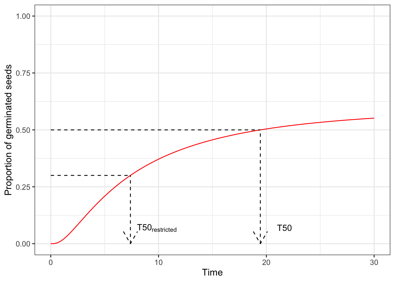
Quantiles and ‘restricted’ quantiles
Due to the presence of the ungerminated/unemerged fraction, quantiles suffer from the intrinsic ambiguity that we could calculate them either for the whole sample, or for the germinated fraction. For example, let’s think that we have a seed lot where the maximum percentage of germination is 60% and thus 40% of seeds are dormant. How do we define the 50^th^ percentile?
In general, we should consider the whole population, including the ungerminated fraction, where the event is not observed; accordingly, the, e.g., 50^th^ percentile (T50) should be defined as the time to 50% germination. Obviously, with such a definition the, e.g., T50 cannot be estimated when the maximum germinated fraction is lower than 50%.
On the other hand, for certain applications, it might be ok to remove the ungerminated fraction prior to estimating the quantiles; in this case, for our example where the maximum germinated fracion is 60%, the T50 would be defined as the time to 30% germination, that is 50% of the maximum germinated fraction.
Due to such an ambiguity, we should talk about quantiles and ‘restricted’ quantiles. The graph below should help clarify such a difference.
As a general suggestion, we should never use restricted quantiles for seed germination/emergence studies, especially when the purpose is to make comparisons across treatment groups (Bradford, 2002; Keshtkar et al. 2021).
Germination/emergence rates
The quantiles of germination times (e.g., T10, T30 or T50) are very common measures of germination velocity, although they may be rather counterintuitive, because a high germination time implies low velocity. Another common measure of velocity is the Germination Rate, that is the inverse of germination time (e.g., GR10 = 1/T10).
The quantiles of germination rates (e.g., GR10, GR30, GR50…) represents the daily progress to germination for a given subpopulation and they are used as the basis for hydro-thermal-time modelling. Therefore, their determination for a seed lot is also very relevant.
Getting the quantiles with ‘drcte’
Parametric models
In a previous post we have used the code below to fit a log-logistic time-to-event model to the germination data for three species of the Verbascum genus:
library(drcte)
library(drcSeedGerm)
data(verbascum)
mod1 <- drmte(nSeeds ~ timeBef + timeAf, fct = LL.3(),
             curveid = Species, data = verbascum)
summary(mod1, units = Dish)
##
## Model fitted: Log-logistic (ED50 as parameter) with lower limit at 0
##
## Robust estimation: Cluster robust sandwich SEs
##
## Parameter estimates:
##
##               Estimate Std. Error  t value  Pr(>|t|)
## b:arcturus   -9.930005   1.111135  -8.9368 4.286e-16 ***
## b:blattaria  -7.198025   0.575290 -12.5120 < 2.2e-16 ***
## b:creticum  -11.033749   0.943374 -11.6961 < 2.2e-16 ***
## d:arcturus    0.356648   0.047915   7.4433 3.715e-12 ***
## d:blattaria   0.840064   0.025593  32.8242 < 2.2e-16 ***
## d:creticum    0.969990   0.017290  56.1015 < 2.2e-16 ***
## e:arcturus   12.059189   0.486010  24.8126 < 2.2e-16 ***
## e:blattaria   4.031763   0.199590  20.2002 < 2.2e-16 ***
## e:creticum    3.200655   0.103161  31.0259 < 2.2e-16 ***
## ---
## Signif. codes:  0 '***' 0.001 '**' 0.01 '*' 0.05 '.' 0.1 ' ' 1
It may be useful to rank the species in terms of their germination velocity and, to that purpose, we could estimate the times to 30% and 50% germination (T30 and T50), that are the 30^th^ and 50^th^ percentiles of the time-to-event distribution. We can use the quantile() method, where the probability levels are passed in as the vector ‘probs’:
quantile(mod1, probs = c(0.3, 0.5))
##
## Estimated quantiles
##
##               Estimate       SE
## arcturus:30%   14.2634 0.992685
## arcturus:50%       NaN      NaN
## blattaria:30%   3.7156 0.106048
## blattaria:50%   4.2536 0.118515
## creticum:30%    2.9759 0.058279
## creticum:50%    3.2187 0.059480
We may note that the T50 is not estimable with Verbascum arcturus, as the maximum germinated proportion (d parameter for the time-to-event model above) is 0.36. Standard errors are obtained by using the delta method and they are invalid whenever the experimental units (seeds) are clustered within containers, such as the Petri dishes.
For all these cases, we should prefer cluster-robust standard errors (Zeileis et al. 2020), which can be obtained by setting the extra argument ‘robust = TRUE’ and providing a clustering variable as the units argument. By setting ‘interval = TRUE’ we can also obtain confidence intervals for the desired probability level (0.95, by default).
quantile(mod1, probs = c(0.3, 0.5), robust = T,
         units = Dish,
         interval = T)
##
## Estimated quantiles
##
##               Estimate       SE   Lower   Upper
## arcturus:30%   14.2634 0.755294 12.7830 15.7437
## arcturus:50%       NaN      NaN     NaN     NaN
## blattaria:30%   3.7156 0.187503  3.3481  4.0831
## blattaria:50%   4.2536 0.209853  3.8423  4.6649
## creticum:30%    2.9759 0.085151  2.8090  3.1428
## creticum:50%    3.2187 0.104743  3.0134  3.4240
We may note that cluster robust standard errors are higher than naive standard errors: the seed in the same Petri dish are correlated and, thus, they do not contribute full information.
If we are interested in the germination rates G30 and G50, we can set the argument ‘rate = T’, as shown in the box below.
quantile(mod1, probs = c(0.3, 0.5), robust = T,
         units = Dish,
         interval = T, rate = T)
##
## Estimated quantiles
##
##               Estimate        SE    Lower    Upper
## arcturus:30%   0.07011 0.0037126 0.062833 0.077386
## arcturus:50%   0.00000 0.0000000 0.000000 0.000000
## blattaria:30%  0.26914 0.0135819 0.242519 0.295759
## blattaria:50%  0.23510 0.0115987 0.212364 0.257830
## creticum:30%   0.33604 0.0096153 0.317191 0.354882
## creticum:50%   0.31069 0.0101106 0.290872 0.330505
Parametric models with environmental covariates
If we have fitted a hydro-thermal time model or other models with an environmental covariate, we can also use the quantile() method, and pass a value for that covariate, as shown in the code below.
# Parametric model with environmental covariate
data(rape)
modTE <- drmte(nSeeds ~ timeBef + timeAf + Psi,
            data = rape, fct = HTLL())
quantile(modTE, Psi = 0,
         probs = c(0.05, 0.10, 0.15, 0.21),
         restricted = F, rate = T, robust = T,
         interval = T)
##
## Estimated quantiles
##
##       Estimate      SE  Lower  Upper
## 1:5%    1.5861 0.22621 1.1428 2.0295
## 1:10%   1.5562 0.21060 1.1435 1.9690
## 1:15%   1.5331 0.20063 1.1399 1.9263
## 1:21%   1.5090 0.19183 1.1330 1.8850
The environmental covariate only accepts a single value; in order to vectorise, we need to use the lapply() function, as shown below.
# This is to vectorise on Psi
psiList <- seq(-1, 0, 0.25)
names(psiList) <- as.character(psiList)
lapply(psiList,
       function(x) quantile(modTE, Psi = x,
                            probs = c(0.05, 0.10, 0.15, 0.21),
                            restricted = F, rate = T,
                            interval = "delta",
                            units = rape$Dish,
                            display = F))
## $`-1`
##         Estimate         SE         Lower      Upper
## 1:5%  0.10860038 0.05566723 -0.0005053802 0.21770614
## 1:10% 0.07869462 0.03741665  0.0053593301 0.15202992
## 1:15% 0.05555279 0.02674484  0.0031338792 0.10797171
## 1:21% 0.03145638 0.01993609 -0.0076176245 0.07053039
##
## $`-0.75`
##        Estimate         SE     Lower     Upper
## 1:5%  0.4779833 0.08302599 0.3152553 0.6407112
## 1:10% 0.4480775 0.06331213 0.3239880 0.5721670
## 1:15% 0.4249357 0.05037871 0.3261952 0.5236762
## 1:21% 0.4008393 0.03876416 0.3248629 0.4768157
##
## $`-0.5`
##        Estimate         SE     Lower     Upper
## 1:5%  0.8473662 0.11816778 0.6157616 1.0789708
## 1:10% 0.8174604 0.09946283 0.6225169 1.0124040
## 1:15% 0.7943186 0.08738918 0.6230390 0.9655982
## 1:21% 0.7702222 0.07670819 0.6198769 0.9205675
##
## $`-0.25`
##       Estimate        SE     Lower    Upper
## 1:5%  1.216749 0.1559175 0.9111565 1.522342
## 1:10% 1.186843 0.1380349 0.9162999 1.457387
## 1:15% 1.163702 0.1265389 0.9156899 1.411713
## 1:21% 1.139605 0.1163701 0.9115239 1.367686
##
## $`0`
##       Estimate        SE    Lower    Upper
## 1:5%  1.586132 0.1947646 1.204400 1.967864
## 1:10% 1.556226 0.1774564 1.208418 1.904034
## 1:15% 1.533084 0.1663240 1.207095 1.859073
## 1:21% 1.508988 0.1564488 1.202354 1.815622
Non-parametric (NPMLE) models
The quantile() method can also be used to make predictions from NPMLE fits. This method works by assuming that the events are evenly scattered within each inspection interval (‘interpolation method’). Inferences need to be explicitly requested by using setting ‘interval = T’; in this case, standard errors are estimated by using a resampling approach, that is performed at the group level, whenever a grouping variable is provided, by way of the ‘units’ argument (Davison and Hinkley, 1997).
mod2 <- drmte(nSeeds ~ timeBef + timeAf, fct = NPMLE(),
             curveid = Species, data = verbascum)
quantile(mod2, probs = c(0.3, 0.5), robust = T, units = Dish,
         interval = T, rate = T)
##
##
##
##
## Estimated quantiles
## (cluster robust bootstrap-based inference)
##
##                 n       Mean   Median        SE   Lower    Upper
## arcturus.30%  999 0.04101624 0.067196 0.0369184 0.00000 0.085956
## arcturus.50%  999 0.00081888 0.000000 0.0074311 0.00000 0.000000
## blattaria.30% 999 0.26973311 0.268949 0.0173015 0.24031 0.303589
## blattaria.50% 999 0.23295275 0.231250 0.0126124 0.21403 0.262669
## creticum.30%  999 0.34452679 0.343750 0.0201617 0.31318 0.382813
## creticum.50%  999 0.30366646 0.302326 0.0125247 0.28282 0.330986
For KDE models, quantiles are calculated from the time-to-event curve by using a bisection method. However, we are still unsure about the most reliable way to obtain standard errors and, for this reason, inferences are not provided with this type of non-parametric models.
Quantiles and Effective Doses (ED)
Quantiles for time-to-event data resamble Effective Doses (ED) for dose-response data, although we discourage the use of this latter term, as the time-to-event curve is a cumulative probability function based on time, that is not a ‘dose’ in strict terms. However, the concept is similar: we need to find the stimulus (time) that permits to obtain a certain response (germination/emergence). Considering such similarity, we decided to define the ED() method for ‘drcte’ objects, that is compatible with the ED() method for ‘drc’ objects. However, for seed germination/emergence data, we strongly favor the use of the quantile() method.
It’s all for this topic; thank you for reading and, please, stay tuned for other posts in this series.
Prof. Andrea Onofri
Department of Agricultural, Food and Environmental Sciences
University of Perugia (Italy)
Send comments to: andrea.onofri@unipg.it
References
- Bradford KJ (2002) Applications of hydrothermal time to quantifying and modeling seed germination and dormancy. Weed Sci 50:248–260
- Davison, A.C., Hinkley, D.V., 1997. Bootstrap methods and their application. Cambridge University Press, UK.
- Keshtkar E, Kudsk P, Mesgaran MB (2021) Perspective: Common errors in dose–response analysis and how to avoid them. Pest Manag Sci 77:2599–2608
- Onofri, A., Mesgaran, M., & Ritz, C. (2022). A unified framework for the analysis of germination, emergence, and other time-to-event data in weed science. Weed Science, 1-13. doi:10.1017/wsc.2022.8
- Zeileis, A., Köll, S., Graham, N., 2020. Various Versatile Variances: An Object-Oriented Implementation of Clustered Covariances in R. J. Stat. Soft. 95. https://doi.org/10.18637/jss.v095.i01