This is the follow-up of a manuscript that we (some colleagues and I) have published in 2016 in the European Journal of Agronomy (Onofri et al., 2016). I thought that it might be a good idea to rework some concepts to make them less formal, simpler to follow and more closely related to the implementation with R. Please, be patient: this lesson may be longer than usual.
First question: what are long-term experiments? Agricultural experiments have to deal with long-term effects of cropping practices. Think about fertilisation: certain types of organic fertilisers may give effects on soil fertility, which are only observed after a relatively high number of years (say: 10-15). In order to observe those long-term effects, we need to plan Long Term Experiments (LTEs), wherein each plot is regarded as a small cropping system, with the selected combination of rotation, fertilisation, weed control and other cropping practices. Due to the fact that yield and other relevant variables are repeatedly recorded over time, LTEs represent a particular class of multi-environment experiments with repeated measures.
The main problem with LTEs: lack of independence
We know that, with linear models, once the effects of experimental factors have been accounted for, the residuals must be independent. Otherwise, inferences are invalid.
With LTEs, observations are repeatedly taken on the same plot and, therefore, the residuals cannot be independent. Indeed, all measurements taken on one specific plot will be affected by the peculiar characteristics of that plot and they will be more alike than measurements taken in different plots. Thus, there will be a ‘plot’ effect, which will induce a within-plot correlation. The problem is: how do we restore the necessary independence of residuals?
At the basic level, the main way to account for the ‘plot’ effect is by including a random term in the model; in this way, we recognise that there is a plot-to-plot variability, following a gaussian distribution, with mean equal to 0 and standard deviation equal to \(\sigma^2_B\) (‘plot’ error). This plot-to-plot variability is additional to the usual residual variability (within-plot error), that is also gaussian with mean equal to 0 and standard deviation equal to \(\sigma^2\).
As the result, if we take one observation, the variance will be equal to the sum \(\sigma^2_B + \sigma^2\). If we take two observations in different plots, they will have different random ‘plot’ effects and, thus, they will be independent. Otherwise, if we take two observations in the same plot, they will share the same random plot effect and they will ‘co-vary’, showing a positive covariance equal to \(\sigma^2_B\). The correlation among observations in the same plot will be quantified by the ratio \(\rho = \sigma^2_B / (\sigma^2_B + \sigma^2)\) (intra-class correlation).
In simple words, adding a random plot effect to the model accounts for the fact that observations in the same plot are correlated. This would be similar to a split-plot design (indeed, we talk about split-plot in time) with the important difference that the sub-plot factor (year) is not randomised. The correlation of observations in one plot will always be the same, independent from the year, which is known as Compound Symmetry (CS) correlation structure. Be careful: it may be more reasonable to assume that observations close in time are more correlated than observations distant in time, but we will address this point elsewhere.
It is necessary to remember that, apart from plots, the experimental design may be characterised by other grouping structures, such as blocks or main plots. All these grouping structures must be appropriately referenced in the model, to account for intra-group correlation. I’ll be back into this in a few moments.
Another problem with LTEs: rotation treatments
In many instances, the aim of LTEs is to compare different cropping systems, which are allocated to different plots, possibly in different blocks. When the different cropping systems involve rotations, we need to consider a very important rule, that was pointed out by W.G. Cochran in a seminal paper dating back to 1937: “The most important rule about rotation experiments is that each crop in the rotation must be grown every year”. If we do not follow this rule, “the experiment has to last longer to obtain equal information on the long-term effects of the treatments” and “the effects of the treatments on the separate crops are obtained under different seasonal conditions, so that a compact summary of the results of the experiment as a whole is made exceedingly difficult”.
The above rule has important consequences: first of all, with, e.g., a three year rotation, we need three plots per treatment and per block in each year, which increases the size of the experiment (that’s why some LTEs are designed without within-year replicates; Patterson, 1964). Secondly, if we want to consider only one crop in the rotation, the experiment becomes unbalanced, as not all plots contribute useful data in each one year. Last, but not least, in long rotations the test crop may return onto the same plot after a relatively long period of time, which may create a totally different correlation structure, compared to short rotations.
How do we build ‘ANOVA-like’ models for LTEs?
For the reasons explained above, building ANOVA-like models for data analyses may be a daunting task and it is useful to follow a structured procedure. First of all, we need to remember that ANOVA models are based on classification variables, commonly known as factors. There are three types of factors:
- treatment factors, which are randomly allocated to randomisation units (e.g. rotations, fertilisations, management of crop residues);
- block factors, which group the observations according to some ‘innate’ (not randomly allocated) criterion (e.g. by position), such as the blocks, the locations, the main-plots, the sub-plots and so on. Block factors may represent the randomisation units, to which treatments are randomly allocated;
- repeated factors, which relate to time and thus cannot be randomised (e.g. years, cycles …).
In order to build a model, the starting point is to list all factors (treatment, grouping and repeated) and their relationships. We can follow the general method proposed by Piepho et al. (2003), which we have slightly modified, to make it more ‘R-centric’. The relationships among factors can be specified by using the following operators:
- the ‘colon’ operator denotes an interaction of crossed effects (e.g. A:B means that A and B are crossed factors);
- the ‘nesting’ operator denotes nested effects (e.g. A/B means that B is nested within A and it is equal to A + A:B);
- the ‘crossing’ operator denotes the full factorial model for two terms (A*B = A + B + A:B).
When building models we need to pay attention to properly code interactions. Let’s have a look at a simple two-way ANOVA, with the ‘JohnsonGrass.csv’ dataset. In this case we have the two crossed effects Length and Timing and we could build a model as: ‘RIZOMEWEIGHT ~ LENGTH + TIMING + LENGTH:TIMING’ that is shortened as: ’RIZOMEWEIGHT ~ LENGTH*TIMING’. However, if we build our model as: ‘RIZOMEWEIGHT ~ LENGTH:TIMING’, the two main effects are ‘absorbed’ by the term ‘LENGTH:TIMING’, which is no longer an interaction. The code below may clear up what I mean.
rm(list=ls())
dataset <- readr::read_csv("https://www.casaonofri.it/_datasets/JohnsonGrass.csv")

mod1 <- lm(RizomeWeight ~ Length + Timing + Length:Timing, data = dataset)
anova(mod1)
## Analysis of Variance Table
##
## Response: RizomeWeight
##               Df  Sum Sq Mean Sq F value    Pr(>F)
## Length         2  1762.2   881.1  9.4795 0.0002961 ***
## Timing         5 16927.9  3385.6 36.4241 3.896e-16 ***
## Length:Timing 10   952.7    95.3  1.0250 0.4354263
## Residuals     54  5019.2    92.9
## ---
## Signif. codes:  0 '***' 0.001 '**' 0.01 '*' 0.05 '.' 0.1 ' ' 1
mod2 <- lm(RizomeWeight ~ Length:Timing, data = dataset)
anova(mod2)
## Analysis of Variance Table
##
## Response: RizomeWeight
##               Df  Sum Sq Mean Sq F value    Pr(>F)
## Length:Timing 17 19642.8 1155.46  12.431 4.766e-13 ***
## Residuals     54  5019.2   92.95
## ---
## Signif. codes:  0 '***' 0.001 '**' 0.01 '*' 0.05 '.' 0.1 ' ' 1
Steps to model building
The steps to model building may be summarised as follows:
- Select the repeated factor.
- Consider one fixed level of the repeated factor and build a treatment model for the randomized treatment factors.
- Consider one fixed level of the repeated factor and build a block model for block factors.
- Check whether randomised treatment factors might interact with block effects: if such an interaction is to be expected it should be added to the model.
- Include the unrandomised repeated factor into the model.
- Combine treatment model and repeated factor model, by crossing or nesting as appropriate.
- Consider which effects in the block model reference randomisation units, i.e. those units which receive the levels of a factor or factor combination by a randomisation process. It should be clear that randomisation units can be seen as randomly selected from a wider population. Therefore, the corresponding terms should be assigned a separate random effect, as explicitly recommended in Piepho (2004).
- Excluding the terms for randomisation units, nest the repeated factor in all the other terms in the block model.
- Combine random effects for randomisation units with the repeated factor, by using the colon operator, in order to derive the correct error terms to accommodate correlation structures.
- Apart from randomisation units (see #7), decide which factors are random and which are fixed. In our examples, the random model will include all random terms for randomisation units (terms at steps 7 and 9), while the fixed model will include all the other terms. Several extensions/changes to this basic approach are possible.
The key idea for the above approach is that for a properly designed experiment, valid analyses should be possible for the data at each single level of the repeated factor. Such a basic requirement should never be taken for granted, but it should be carefully checked before the beginning of the model building process (see later for Example 3).
Some further definitions
It is perhaps important to clear up some definitions, which we will use afterwards. Each crop component in a rotation is usually known as a phase; e.g., in the rotation Maize-Wheat-Wheat, Maize is phase 1, Wheat is phase 2 and Wheat is phase 3. The number of phases defines the period (duration) of the rotation. All phases need to be contemporarily present in any one year and, therefore, we can define the so-called sequences: i.e. each of the \(n\) possible arrangements for a rotation of \(n\) years, having the same crop ordering, but different initial phases (e.g Maize - Wheat - Wheat, Wheat - Wheat - Maize and Wheat - Maize - Wheat). Each sequences is uniquely identified by its starting phase, which needs to be randomly allocated to each plot at the start of the experiment.
Examples
In order to give a practical demonstration, we have selected five exemplary datasets, relating to LTEs with different designs. If you are in a hurry, you can follow the links below to jump directly to the example that is most relevant for you.
- Example 1. LTEs to compare monocultures or perennial crops
- Example 2. LTEs to compare rotations of the same length and one test crop per rotation cycle
- Example 3. LTEs with a fixed rotation (one test crop per cycle) and different treatments
- Example 4. LTE with a fixed rotation, different treatments and more than one phase per crop and cycle
- Example 5. LTEs with several rotations of different lengths and different number of phases per crop and rotation cycle
We will analyse all examples, using the ‘tidyverse’ (Wickham, 2019) for data management and the ‘nlme’ package to fit random effect models (Pinheiro et al., 2019). We will also use the ‘asreml-R’ (Butler, 2019) package, for those of you who own a licence. Let’s load those packages in the R environment.
rm(list = ls())
library(tidyverse)
library(nlme)
# library(asreml)
Example 1: LTEs with monocultures or perennial crops
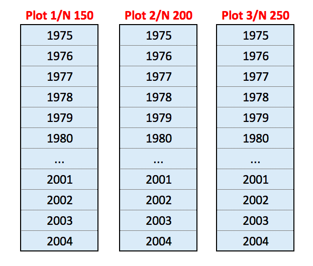
Wheat is grown in continuous cropping from 1983 to 2012, with three fertilisation levels (150, 200 and 250 kg N ha\(^{-1}\)), randomly assigned to three plots in each of three blocks. In all, there are nine plots with yearly sampling, with a total of 270 wheat yield observations in 30 years. The following figure shows the design for one block: the spatial split for each plot represents the actual temporal split.
For this example, the repeated factor is the year (YEAR). In one year, the treatment factor is nitrogen fertilisation (N) and there are two block factors, i.e. the blocks (BLOCK) and the plots within each block (PLOT). Therefore, the block model is BLOCK + BLOCK:PLOT.
We now introduce the repeated factor YEAR and combine it with the treatment model, by including N*YEAR = N + YEAR + N:YEAR. The term BLOCK:PLOT references the randomisation units and receives a random effect. As the year might interact with the block, we add the term BLOCK:YEAR. We also combine the year with the random effect for plots (BLOCK:PLOT:YEAR), although this residual term does not need to be explicitly coded when implementing the model. The final model is (the operator ~ means ‘is modelled as’):
YIELD ~ N + BLOCK + YEAR + N:YEAR + BLOCK:YEAR
RANDOM = BLOCK:PLOT + BLOCK:PLOT:YEAR
Now we can use the above notation in R, as shown in the box below.
rm(list=ls())
dataset <- read_csv("https://www.casaonofri.it/_datasets/LTE1.csv")

dataset <- dataset %>%
  mutate(across(c(Block, Plot, Year, N), factor))
head(dataset)
## # A tibble: 6 × 5
##   Plot  N     Year  Block Yield
##   <fct> <fct> <fct> <fct> <dbl>
## 1 33    fn150 1983  1      4.54
## 2 98    fn150 1983  3      4.18
## 3 162   fn150 1983  2      3.7
## 4 33    fn150 1984  1      4.57
## 5 98    fn150 1984  3      5.04
## 6 162   fn150 1984  2      5.06
# Implementation with lme
mod <- lme(Yield ~ Block + Year + N + N:Year + Block:Year,
           random = ~ 1|Plot, data = dataset)
anova(mod)
##             numDF denDF  F-value p-value
## (Intercept)     1   116 5434.427  <.0001
## Block           2     4    0.300  0.7564
## Year           29   116   36.496  <.0001
## N               2     4    1.304  0.3664
## Year:N         58   116    1.663  0.0105
## Block:Year     58   116    2.545  <.0001
# Implementation with asreml (the residual statement is unnecessary, here)
# Need to sort the data according to the residual statement
# datasetS <- dataset %>%
#  arrange(Plot, Year)
# mod <- asreml(Yield ~ Block + Year + N + N:Year + Block:Year,
#           random = ~ Plot,
#           residual = ~ Plot:Year, data = datasetS)
# wald(mod)
It is worth to notice that the same model may be fitted in an alternative way, i.e. by dropping the BLOCK:PLOT random effects and using the residual term BLOCK:PLOT:YEAR to accommodate the CS structure into the model. This may be done very intuitively with ‘asreml’, by using the following notation:
# Code not run
# mod <- asreml(Yield ~ Block + Year + N + N:Year + Block:Year,
#           residual = ~ Plot:cor(Year), data = datasetS)
# summary(mod)$varcomp
We see that the final command returns the correlation between observations in the same plot. With ‘lme’ package, the notation is different, as we have to switch from the ‘lme()’ to the ‘gls()’ function:
mod <- gls(Yield ~ Block + Year + N + N:Year + Block:Year,
           correlation = corCompSymm(form = ~1|Plot), data = dataset)
mod$modelStruct$corStruct
## Correlation structure of class corCompSymm representing
##       Rho
## 0.1269864
This alternative coding can be used to implement different correlation structures for the cases when a simple CS correlation structure is not satisfactory. For example, when the observations close in time are more correlated than those distant in time, we can implement a serial correlation structure by appropriately changing the ‘residual’ argument in ‘asreml()’ or the ‘correlation’ argument in ‘lme()’.
Example 2. LTEs with different rotations of the same length and one test crop per rotation cycle
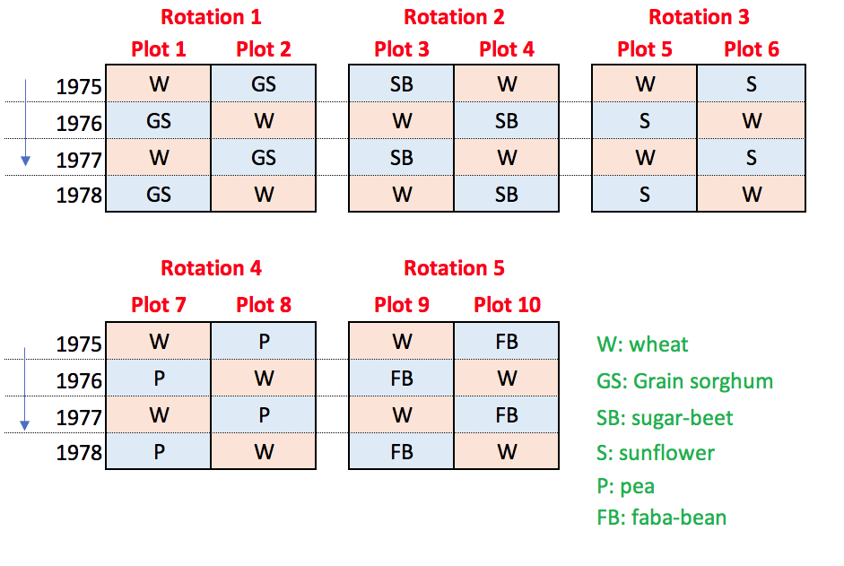
Wheat is grown in five types of two-year rotations, with either pea (Pisum sativum L), grain sorghum (Sorghum bicolor (L.) Moench), sugar beet (Beta vulgaris L. subsp. saccharifera), sunflower (Helianthus annuus L.) and faba bean (Vicia faba L. subsp. minor). For each rotation, there are two possible sequences (wheat in odd years and wheat in even years) and the ten combinations (five rotations by two sequences) are completely randomised to ten plots per each of three blocks (Figure 2). Therefore, five wheat plots out of the available ten plots are used from each block and year, for a total of 450 observations, from 1983 to 2012. The experimental design for one block is shown in the figure below.
In this example we have two crops in a rotation and both crops are grown in different plots in the same year. Thus, for each rotation, we have two sequences in time (e.g., maize-sunflower and sunflower-maize). If we consider only one of the two crops, the main difference with respect to Example 1 is that the data obtained in two consecutive years for the same treatment and block are independent, in the sense that they are obtained in different plots. Otherwise, data obtained in a two-year interval (on different rotation cycles) on the same block are correlated, as they originate from the same plot.
Which is the repeated factor? Indeed, if we look only at one phase in the rotation (in this case wheat), we note that observations are repeated every second year on the same plot (Figure above), according to the sequence they belong to. In other words, observations are repeated on each rotation cycle (CYC; two years) in the same plot, while there is neither a within-cycle repetition nor a within-cycle phase difference: we have only one observation per plot per cycle. Therefore, it is natural to take the rotation cycle as the repeated factor (CYC instead of YEAR).
As the next step, we should look at what happens in one fixed level of CYC: what did we randomize to the ten plots in a two-years time slot? It is clear that, considering only wheat, we randomised each combination of rotation (ROT) and positioning in the sequence (SEQ; i.e. wheat as the first crop of the sequence and wheat as the second crop of the sequence). Therefore, the treatment factors are ROT and SEQ. Now we can cross the repeated factor with the treatment factors. Accordingly, The model is:
YIELD ~ SEQ*ROT + BLOCK + CYC + ROT:CYC + BLOCK:CYC
RANDOM: BLOCK:PLOT + BLOCK:PLOT:CYC
The code below shows how to fit the model with R.
rm(list=ls())
dataset <- read_csv("https://www.casaonofri.it/_datasets/LTE2.csv")

dataset <- dataset %>%
  mutate(across(c(1:7), factor))
head(dataset)
## # A tibble: 6 × 8
##   Block Main  Plot  Rot   Year  Sequence Cycle Yield
##   <fct> <fct> <fct> <fct> <fct> <fct>    <fct> <dbl>
## 1 1     1_1   4     SBW   1983  1        1      5.1
## 2 3     3_1   70    SBW   1983  1        1      4.5
## 3 2     2_1   135   SBW   1983  1        1      4.53
## 4 1     1_0   27    SBW   1984  0        1      5.83
## 5 3     3_0   95    SBW   1984  0        1      6.26
## 6 2     2_0   160   SBW   1984  0        1      6.22
# Implementation with lme
mod <- lme(Yield ~ Block + Rot*Sequence + Block:Sequence +
             Cycle + Cycle:Sequence + Rot:Cycle +
             Rot:Sequence:Cycle + Cycle:Block +
             Cycle:Block:Sequence,
             random = ~1|Plot,
           data = dataset)
anova(mod)
##                      numDF denDF   F-value p-value
## (Intercept)              1   224 115809.71  <.0001
## Block                    2    16     42.68  <.0001
## Rot                      4    16      4.19  0.0165
## Sequence                 1    16     26.14  0.0001
## Cycle                   14   224    133.43  <.0001
## Rot:Sequence             4    16      3.60  0.0283
## Block:Sequence           2    16      2.24  0.1384
## Sequence:Cycle          14   224    119.86  <.0001
## Rot:Cycle               56   224      1.74  0.0025
## Block:Cycle             28   224      8.77  <.0001
## Rot:Sequence:Cycle      56   224      1.61  0.0081
## Block:Sequence:Cycle    28   224      6.85  <.0001
This approach is commonly suggested in literature (see Yates, 1954) and it is convenient, mainly because the resulting model is orthogonal and may be fitted by ordinary least squares. Indeed, for Dataset 2 (and similar experiments), there is only one observation for each block, treatment, cycle, sequence and no missing data (in our case: 3 blocks x 5 rotations x 2 sequences x 15 cycles = 450 observations). The phase should not enter into this model, as we are looking only at one of the two crops (only one phase).
However, the drawback is that such an approach cannot be immediately extended to the other more complex examples (e.g. rotations with different lengths and/or with a different number of test-crops). Furthermore, the effect of years is partitioned into three components, i.e. ‘cycles’, ‘sequences’ and ‘cycle x sequences’, which might make modeling possible ‘fertility’ trends over time less immediate. In this respect, we should note that possible differences between sequences for a given cycle (wheat as the first crop of the sequence and wheat as the second crop of the sequence, i.e. wheat in even years and wheat in odd years) do not carry any meaning that helps understand the behaviour of rotations.
An alternative and more natural approach is to take the year as the repeated factor; indeed, for Example 2, the year effect is totally confounded with the factorial combination of ‘cycle’ and ‘sequence’ (15 cycles x 2 sequences = 30 years). If we consider the YEAR as the repeated factor, in one year the treatment model is composed only by the rotation (ROT), that is allocated to plots (PLOT), within blocks. The block model for one year is BLOCK/PLOT = BLOCK + BLOCK:PLOT. We can combine the treatment model with the repeated factor (ROT:YEAR) and add the term BLOCK:YEAR. The final model is:
YIELD ~ ROT + BLOCK + YEAR + ROT:YEAR + BLOCK:YEAR
RANDOM: BLOCK:PLOT + BLOCK:PLOT:YEAR
Apart from random effects for randomisation units, this model is totally similar to the one used for multi-environment genotype experiments and, represents a convenient and clear platform for the analyses of LTE data. We remind the reader that the residual term (BLOCK:PLOT:YEAR) does not need to be explicitly coded when implementing the model.
# Implementation with lme
mod <- lme(Yield ~ Block + Rot + Year + Rot:Year + Block:Year,
             random = ~1|Plot,
           data = dataset)
This gives us a good common modelling platform for all datasets, although it may be argued that the models are no longer orthogonal, as not all plots produce data in all years. It should be recognised, however, that the lack of orthogonality can easily be accommodated within mixed models.
The situation is totally different if we look at both the phases of the rotation (e.g. wheat and sunflower): in this case, we have a phase difference within each cycle and, considering one level of the repeated factor year, the treatment model should contain both the rotation and the phase, together with their interaction. When we introduce the year (steps 5 and 6 above), we also introduce the interactions ‘year x rotation’, ‘year x phase’ and ‘year x rotation x phase’, which are all meaningful when studying the behaviour of rotations.
Example 3. LTEs with a fixed rotation (one test crop per cycle) and different treatments
Durum wheat (Triticum durum L.) is grown in a two-year rotation with a spring crop and nine cropping systems, consisting of the factorial combination of three soil tillage methods (CT: conventional 40 cm deep ploughing; M: scarification at 25 cm; S: sod seeding with chemical desiccation and chopping) and three N-fertilisation levels (N0, N90 and N180, corresponding to 0, 90 and 180 kg N \(ha^{-1}\)). The two possible rotation sequences (wheat-spring crop and spring crop-wheat) are arranged in two adjacent fields, which therefore host the two different crops of the rotation in the same year. Within the two fields, there are two independent randomisations, each with two blocks, tillage levels randomised to main-plots (1500 \(m^2\)) and N levels randomised to sub-plots (500 \(m^2\)), according to a split-plot design with two replicates. The design is taken from Seddaiu et al. (2016), while the data have been simulated by using Monte Carlo methods.
This type of LTE is very similar to the previous one, though we have a different experimental layout:
- there are two experimental treatments, laid out in a split-plot design;
- the two sequences are accommodated in two fields.
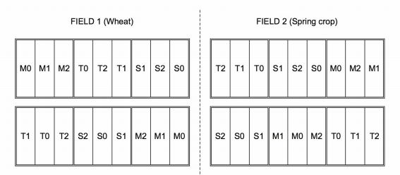
The experimental design for Dataset 3, for each of two fields in one year is reported in the figure below. The position of wheat and spring crop is exchanged in the following year (CT: conventional ploughing; M: scarification; S: sod seeding; 0: no nitrogen fertilisation; 1: 90 kg N \(ha^{-1}\); 2: 180 kg N \(ha^{-1}\)).
Before proceeding to model building for Example 3, we need to discuss whether valid analyses are possible at each single level of the repeated factor. Indeed, this is clearly true if we take the year as the repeated factor and consider only one of the two crops in the rotation (wheat, in this case). However, if we intended to consider both crops and compare e.g. their yields, the crop effect would be confounded with the field effect within a single year and, therefore, valid within-year analyses would not be possible. In this case, we should resort to taking the rotation cycle as the repeated factor.
Dealing only with wheat, we can therefore take the YEAR as the repeated factor and consider that, in one year, the randomised treatment factors are tillage (T) and nitrogen fertilisation (N) and the treatment model is T + N + T:N.
The block factors are the FIELDS, the BLOCKS within fields, the MAIN plots within blocks and the subplots (SUB) within main plots. The block model (for one year) is FIELD + FIELD:BLOCK + FIELD:BLOCK:MAIN + FIELD:BLOCK:MAIN:SUB.
The treatment and repeated model can be combined as: (T + N + T:N)*YEAR = T + N + T:N + YEAR + T:YEAR + N:YEAR + T:N:YEAR.
At this stage, the FIELD main effect needs to be removed, as it is totally confounded with the years. We assign a random effect to the other randomisation units, i.e. FIELD:BLOCK, FIELD:BLOCK:MAIN and FIELD:BLOCK:MAIN:SUB and combine these random terms with the repeated factor YEAR, by using the colon operator, which leads us to:
YIELD ~ T + N + T:N + YEAR + T:YEAR + N:YEAR + T:N:YEAR
RANDOM: FIELD:BLOCK + FIELD:BLOCK:MAIN + FIELD:BLOCK:MAIN:SUB + FIELD:BLOCK:YEAR + FIELD:BLOCK:MAIN:YEAR + FIELD:BLOCK:MAIN:SUB:YEAR
As usual, the last term (residual) does not need to be explicitly included when implementing the model, but it can be used, together with the two previous ones (FIELD:BLOCK:YEAR + FIELD:BLOCK:MAIN:YEAR) to accommodate possible serial correlation structures into the model, by allowing year-specifity of all design effects and the residuals. For this types of models with several crossed random effects, the coding of ‘lme()’ is not straightforward and it does not always lead to a flexible implementation of correlation structures.
In the code below we need to build dummy variables for all random effects (five variables, excluding the residual error term, which is not needed). Afterwards, we have to code the random effects as a list; R expects that the element of such list are nested and, therefore, we need to work around this by coding an additional variable, which takes the value of ‘1’ for all subjects, so that the nesting structure is only artificial. We use the ‘pdIdent’ construct to say that each random effect is homoscedastic and uncorrelated.
rm(list=ls())
dataset <- read_csv("https://www.casaonofri.it/_datasets/LTE3.csv")
dataset <- dataset %>%
  mutate(across(c(1:9), factor)) %>%
  mutate(FB = factor(Block:Field),
         FBM = factor(FB:Main),
         FBMS = factor(FBM:Sub),
         FBY = factor(FB:Year),
         FBMY = factor(FBM:Year),
         one = 1L)

mod <- lme(Yield ~ T + N + N:T +
                 Year + Year:T + Year:N + Year:N:T,
                 random = list(one = pdIdent(~FB - 1),
                               one = pdIdent(~FBM - 1),
                               one = pdIdent(~FBMS - 1),
                               one = pdIdent(~FBY - 1),
                               one = pdIdent(~FBMY - 1)),
               data = dataset, na.action = na.omit)

# Fixed effects tested by using LRT
library(car)
Anova(mod)
## Analysis of Deviance Table (Type II tests)
##
## Response: Yield
##             Chisq Df Pr(>Chisq)
## T          5.1169  2    0.07743 .
## N        804.1717  2  < 2.2e-16 ***
## Year     446.6794 17  < 2.2e-16 ***
## T:N        6.2105  4    0.18397
## T:Year   142.5132 34  3.065e-15 ***
## N:Year   246.5584 34  < 2.2e-16 ***
## T:N:Year 159.3230 68  2.705e-09 ***
## ---
## Signif. codes:  0 '***' 0.001 '**' 0.01 '*' 0.05 '.' 0.1 ' ' 1
The fit takes a long time and it is not easy to manipulate the model to introduce correlation structures for the random effects. However, it is not difficult to introduce the correlation of residuals, by using the ‘correlation’ argument (see above).
Coding the same model with ‘asreml()’ is easier and so is to introduce patterned correlations structures. However, the design has to be balanced and, therefore, we need to introduce NAs for missing observations.
# Asreml fit (not run)
# datasetS <- dataset %>%
#  arrange(Sub, Year)
# mod2 <- asreml(Yield ~ T + N + N:T +
#                 Year + Year:T + Year:N + Year:N:T,
#                 random = ~FB + FB:Main + FB:Main:Sub +
#                 FB:Year + FB:Main:Year,
#               residual = ~ Sub:Year,
#               data = datasetS)
# summary(mod2)$varcomp
Example 4. LTE with a fixed rotation, different treatments and more than one phase per crop and cycle
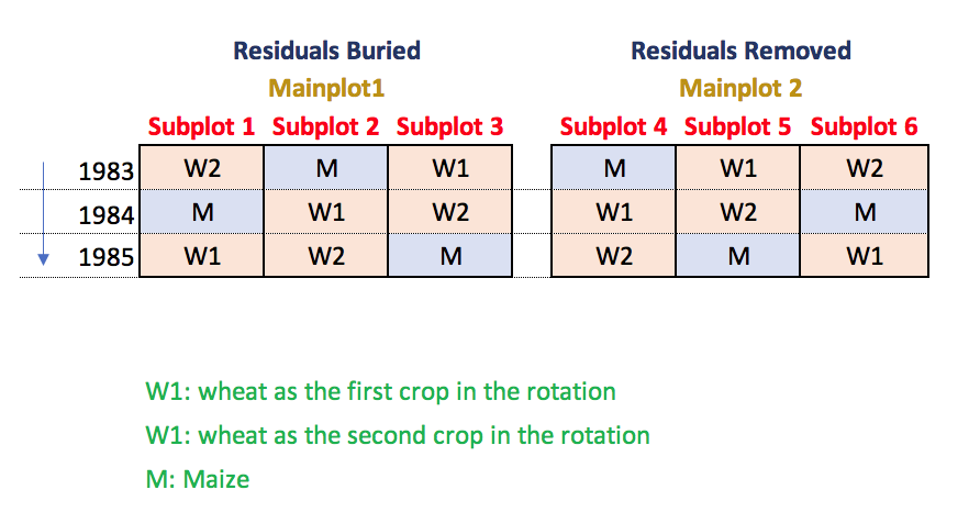
Wheat is grown in a three-year rotation maize-wheat-wheat, under two types of management of crop residues (burial and removal), which are randomised to main plots, while the three possible rotation sequences are randomised to subplots. This experiment has 18 plots (three sequences x two treatment levels x three blocks) and, in every year, 12 of those are cropped with wheat and six with maize.
Also in this case, the response variable is wheat yield from 1983 to 2012, i.e. twelve observations per year and 360 observations in total. Data obtained in the same plot in different years belong to two different phases (wheat after maize and wheat after wheat; the experimental design for one block is shown in the figure below).
With respect to Example 3, the situation becomes more complex, because we have two distinct phases in each rotation cycle (phase difference: wheat after maize and wheat after wheat). As usual, we start by regarding the YEAR as the repeated factor. In one year, the treatment factors are the management of soil residues (RES, that is randomly allocated to main-plots) and the phases (P; randomly allocated to subplots); the treatment model is indeed: RES*P.
In one year, the block model is: BLOCK/MAIN/SUB = BLOCK + BLOCK:MAIN + BLOCK:MAIN:SUB. Introducing the YEAR as repeated factor, we can combine the treatment model with the repeated model as: RES + P + RES:P + YEAR + RES:YEAR + P:YEAR + RES:P:YEAR.
The terms BLOCK:MAIN and BLOCK:MAIN:SUB reference randomisation units and should receive random effects. The blocks may interact with the years (BLOCK:YEAR), while the random effects for randomisation units can be made year-specific by adding BLOCK:MAIN:YEAR and the residual term BLOCK:MAIN:SUB:YEAR. The final model is:
YIELD ~ RES + P + RES:P + YEAR + RES:YEAR + P:YEAR + RES:P:YEAR + BLOCK + BLOCK:YEAR
RANDOM: BLOCK:MAIN + BLOCK:MAIN:SUB + BLOCK:MAIN:YEAR + BLOCK:MAIN:SUB:YEAR
rm(list=ls())
dataset <- read_csv("https://www.casaonofri.it/_datasets/LTE4.csv")
dataset <- dataset %>%
mutate(across(c(1:7), factor)) %>%
mutate(Main = factor(Block:Res),
Sub = factor(Main:Sub))
mod <- lme(Yield ~ Block + Res*P +
Year + Year:Res + Year:P + Year:Res:P +
Block:Year,
random = list(Main = pdIdent(~1),
Main = pdIdent(~Sub - 1),
Main = pdIdent(~Year - 1)),
data = dataset)Example 5: LTEs with several rotations of different lengths and different number of phases per crop and rotation cycle
Wheat is grown in five maize (M) - wheat (W) rotations of different lengths, i.e. M-W, M-W-W, M-W-W-W, M-W-W-W-W, M-W-W-W-W-W. For all rotations, all phases are contemporarily present in each year, for a total of 20 plots (one for each of the possible sequences, i.e. 2 + 3 + 4 + 5 + 6 = 20) in each of three blocks. Considering wheat yield as the response variable, we find that only 15 observations are obtained in each year, for a total of 1350 data, from 1983 to 2012.
Experiments of this type represent a high degree of complexity. Indeed, in contrast to all other examples, after 30 years there are plots with: (i) a different number of observations for the same test crop; (ii) a different number of cycles (in some cases the last cycle is also incomplete); (iii) a different number of phases for wheat.
In some cases, it is necessary to compare several rotations with different characteristics (e.g. a different duration and/or a different number of tests crops and /or a different number of phases per crop), which may create a complex design with some degree of non-orthogonality.
The repeated factor is again the YEAR. In one year, the treatment factors are the rotation system (ROT) and the rotation phase (P), which are randomly allocated to plots. As there is a different number of phases for each rotation, we nest the phase within the rotation, leading to the following treatment model: ROT/P = ROT + P:ROT.
In one year, the block model is BLOCK/PLOT = BLOCK + BLOCK:PLOT. The repeated factor is included and combined with the treatment model, by introducing YEAR + ROT:YEAR + ROT:P:YEAR.
The term BLOCK:PLOT references randomisation units and needs to receive a random effect, while the term YEAR:BLOCK can be added to the model, together with the residual term BLOCK:PLOT:YEAR. The final model is:
YIELD ~ ROT + P:ROT + YEAR + ROT:YEAR + ROT:P:YEAR
RANDOM: BLOCK:PLOT + BLOCK:PLOT:YEAR
In the implementation below we did not succeed reaching convergence with ‘lme()’, but we were successful ‘with asreml()’.
rm(list=ls())
dataset <- read_csv("https://www.casaonofri.it/_datasets/LTE5.csv")

dataset <- dataset %>%
  mutate(across(c(1:7), factor))

# mod <- asreml(Yield ~ Block + Rot + Rot:P +
#                 Year + Year:Rot + Year:Rot:P + Block:Year,
#               random = ~Plot,
#               data = dataset)

# mod <- lme(Yield ~ Block + Rot + Rot:P +
#                Year + Year:Rot + Year:Rot:P + Block:Year,
#                random=~1|Plot,
#              data = dataset)
Warning!
Models 1 to 5 are fairly similar and they are very closely related to those used for multi-environment experiments. However, there are some peculiar aspects which needs to be taken under consideration.
- Apart from Dataset 1, there is always a certain degree of unbalance, as plots do not produce data every year. Testing for fixed effects requires great care.
- In all cases, the model formulations shown above induce a compound symmetry correlation structure for observations taken in the same plot over time (‘split-plot in time’). This is seldom appropriate and, thus, more complex correlations structures should be considered.
- In the above formulations, only randomisation units have been given a random effect, while all the other effects have been regarded as fixed. Obviously, depending on the aims of the analyses, it might be convenient and appropriate to regard some of these effects (e.g., the year main effect and interactions) as random.
It’s all, thanks for reading this far. If you have any comments, please, drop me a note at andrea.onofri@unipg.it. Best wishes,
Prof. Andrea Onofri
Department of Agricultural, Food and Environmental Sciences
University of Perugia (Italy)
References
- Brien, C.J., Demetrio, C.G.B., 2009. Formulating mixed models for experiments, including longitudinal experiments. Journal of Agricultural, Biological and Environmental Statistics 14, 253–280.
- David Butler (2019). asreml: Fits the Linear Mixed Model. R package version 4.1.0.110. www.vsni.co.uk
- Cochran, W.G., 1939. Long-Term Agricultural Experiments. Supplement to the Journal of the Royal Statistical Society 6, 104–148.
- Onofri, A., Seddaiu, G., Piepho, H.-P., 2016. Long-Term Experiments with cropping systems: Case studies on data analysis. European Journal of Agronomy 77, 223–235.
- Patterson, H.D., 1964. Theory of Cyclic Rotation Experiments. Journal of the Royal Statistical Society. Series B (Methodological) 26, 1–45.
- Payne, R.W., 2015. The design and analysis of long-term rotation experiments. Agronomy Journal 107, 772–785.
- Piepho, H.-P., Büchse, A., Emrich, K., 2003. A Hitchhiker’s Guide to Mixed Models for Randomized Experiments. Journal of Agronomy and Crop Science 189, 310–322.
- Piepho, H.-P., Büchse, A., Richter, C., 2004. A Mixed Modelling Approach for Randomized Experiments with Repeated Measures. Journal of Agronomy and Crop Science 190, 230–247.
- Pinheiro J, Bates D, DebRoy S, Sarkar D, R Core Team (2019). nlme: Linear and Nonlinear Mixed Effects Models. R package version 3.1-142, <URL: https://CRAN.R-project.org/package=nlme>.
- Seddaiu, G., Iocola, I., Farina, R., Orsini, R., Iezzi, G., Roggero, P.P., 2016. Long term effects of tillage practices and N fertilization in rainfed Mediterranean cropping systems: durum wheat, sunflower and maize grain yield. European Journal of Agronomy 77, 166–178. https://doi.org/10.1016/j.eja.2016.02.008
- Wickham et al., (2019). Welcome to the tidyverse. Journal of Open Source Software, 4(43), 1686, https://doi.org/10.21105/joss.01686.