Simple data analyses with germination indices
Andrea Onofri
10 December, 2018
Introduction
Summarising the results of germination assays by using germination indices is still a very widespread practice. Several indices exist, which have been throughly reviewed by Ranal and Santana (2006). In an early series of two papers, Brown and Meyer stated that no single index can unambiguously combine the three main features of seed germination (i.e. uniformity, speed and extent) in one single value. Therefore, they concluded that the best approach to data analyses is to use the observed germination data to fit a germination curve, which can be used to describe the whole time-course of germination. If a close fit is obtained, the germination curve can be summarised by using a few derived coefficients.
The above authors suggest the use of non-linear regression, which has become a rather widespread method in literature to derive germination indices from germination curves. Recently, such an approach has been also implemented in the R package ‘germinationmetrics’ (Aravind et al., 2018). We concur with the curve-fitting suggestion, although we argue that non-linear regression is not the correct fitting method, as shown in previous papers by several authors, including ourselves (Hay et al., 2014; Hunter et al., 1984; McNair et al., 2012; Onofri et al., 2018, 2010, 2011, 2014; Ritz et al., 2013; Scott et al., 1984).
The aim of this work was to consistently reassess the calculation of germination indices within the time-to-event modelling platform, which has already proven useful to account for all peculiarities of seed germination data (including censoring), resulting in reliable estimates of parameters and standard errors. We have also implemented the proposed approach within an user-friendly R package, to make it largely available among seed scientists.
#The example
This dataset was taken from previously published work (Pace and Benincasa, 2010). Seeds of rapeseed (Brassica napus L. var. oleifera, cv. Excalibur) were tested in Petri dishes at different water potentials (-0.03, -0.15, -0.3, -0.4, -0.5, -0.6, -0.7, -0.8, -0.9, -1, -1.1, -1.2, -1.5 MPa), which were created by using a polyethylene glycol solution (PEG 6000). For each water potential level, three replicated Petri dishes with 50 seeds each were incubated at 20 C. Germinated seeds were counted and removed every 2-3 days for 14 days. We have already analysed this dataset in a previous paper, where we used it to fit a hydro-time-to-event model (Onofri et al., 2018). In this case, we propose a different type of analysis, where we aim at obtaining some relevant germination indices per each Petri dish, to be submitted to further analyses. In particular, we would like to obtain:
- the germination rate for the 10th, 30th and 50th percentile (GR10, GR30 and GR50);
- the maximum germinated proportion.
The dataset is available within the package ‘drcSeedGerm’; the following code loads the package and dataset; if necessary, the ‘drcSeedGerm’ package needs to be installed from github (follow the link above to home page).
library(drcSeedGerm)
data(rape)
head(rape, 10)
##    Psi Dish timeBef timeAf nSeeds nCum propCum
## 1    0    1       0      3     49   49    0.98
## 2    0    1       3      4      0   49    0.98
## 3    0    1       4      5      0   49    0.98
## 4    0    1       5      7      0   49    0.98
## 5    0    1       7     10      0   49    0.98
## 6    0    1      10     14      0   49    0.98
## 7    0    1      14    Inf      1   NA      NA
## 8    0    2       0      3     47   47    0.94
## 9    0    2       3      4      0   47    0.94
## 10   0    2       4      5      0   47    0.94
As we see, the dataset is organised, as necessary for fitting a time-to-event model with the function ‘drm()’ in the ‘drc()’ package (Ritz et al., 2015). In order to get germination indices, we propose that a time-to-event model is fit to each Petri dish and the relevant indices are retreived from the model fit. In particular, if we fit a log-based model in ‘drc’ (i.e. ‘LL.3()’, ‘W1.3()’ or ‘W2.3()’), we could retreive the maximum germinated proportion as the parameter ‘d’ and the GR-values as the inverse og germination times, as obtained by using the ‘ED()’ function. We show an example with the 23-th Petri dish.
library(drc)
mod <- drm(nSeeds ~ timeBef + timeAf, fct = LL.3(),
  data = rape, subset = c(Dish == 23),
  type = "event")
summary(mod)
##
## Model fitted: Log-logistic (ED50 as parameter) with lower limit at 0 (3 parms)
##
## Parameter estimates:
##
##                Estimate Std. Error t-value   p-value
## b:(Intercept) -3.156943   0.707664 -4.4611 8.155e-06 ***
## d:(Intercept)  0.985926   0.020877 47.2261 < 2.2e-16 ***
## e:(Intercept)  2.778121   0.259362 10.7114 < 2.2e-16 ***
## ---
## Signif. codes:  0 '***' 0.001 '**' 0.01 '*' 0.05 '.' 0.1 ' ' 1
plot(mod, log="", ylim=c(0,1))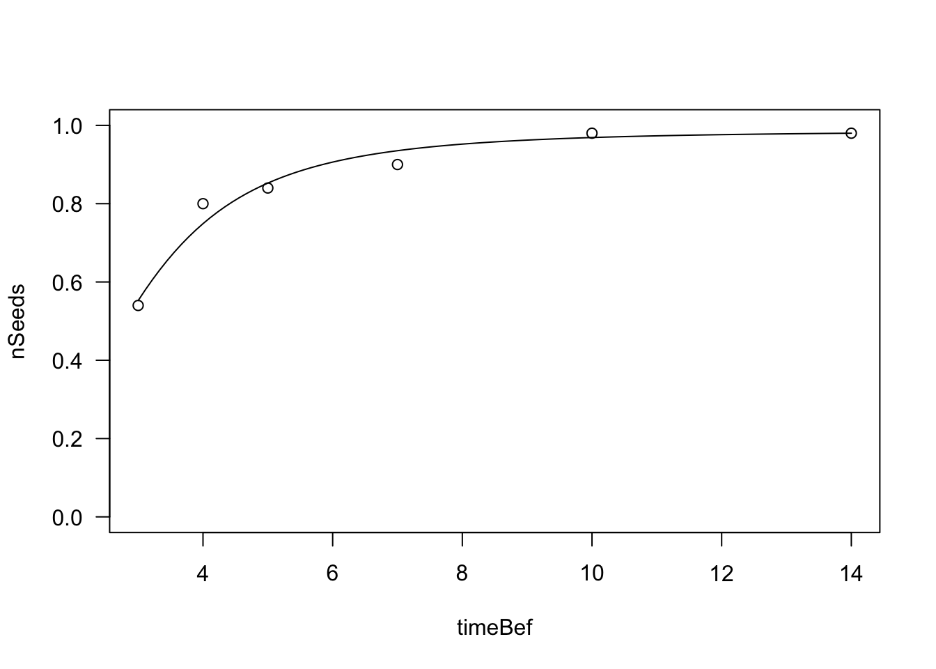
ED(mod, c(0.1, 0.3, 0.5), type = "absolute")
##
## Estimated effective doses
##
##         Estimate Std. Error
## e:1:0.1  1.39204    0.28965
## e:1:0.3  2.13788    0.27192
## e:1:0.5  2.80336    0.25969
Please, note that I used the ‘type = “absolute”’ argument to the ‘ED()’ function. I wanted to retreive the time to germinations for the 10th, 30th and 50th percentiles, considering the whole seed population and not only the germinated fraction. This is usually considered more appropriate by seed biologists. Germination rates can be obtained as the reciprocal of germination times and standard errors can be obtained by using the delta method; I will not give an example, as it is not needed, here.
The problem now is how to automate the process and calculate these germination indices for all Petri dishes. If we go through the dataset, we see that only a few Petri dishes show a clear germination time-course that would allow a three-parameter log-logistic model to be succesfully fit. Indeed, there might be five different situations:
- dishes with no or negligible germination (e.g. less than 10%)
- dishes where the maximum germinated proportion is reached already at the first germination time
- dishes not included in 1 or 2, but where, nonetheless, germination models cannot be succesfully fit.
- dishes with complete germination, where a three-parameter logistic is overparameterised and gives convergence problems. However, a two-parameter logistic (‘LL.2()’) can be succesfully fit
- dishes where a three-parameter logistic can be succesfully fit.
For the cases 1, 2 and 3 we might still be able to estimate maximum germinated proportion, germination times and germination rates. Indeed, if our bioassay has been long enough to observe all possible germinations, we could take the final observed germinated proportion. Furthermore, we can obtain germination rates and times by using the non-parametric equations given in Aravind et al. (2018). For these estimators, bootstrap standard errors may be easily obtained by resampling the seeds in each Petri dish.
I have automated this process within the ‘drmSG()’ function in the ‘drcSeedGerm’ package and would like to give an example. Please, note that ‘drmSG()’ is just a wrapper to the ‘drm()’ function and uses a similar syntax.
mod <- drmSG(nSeeds ~ timeBef + timeAf, curveid = Dish,
                       data=rape, fct = "LL", g = c(10, 30, 50))
## Error in optim(startVec, opfct, hessian = TRUE, method = optMethod, control = list(maxit = maxIt,  :
##   non-finite finite-difference value [2]
## Error in optim(startVec, opfct, hessian = TRUE, method = optMethod, control = list(maxit = maxIt,  :
##   non-finite finite-difference value [2]
## Error in optim(startVec, opfct, hessian = TRUE, method = optMethod, control = list(maxit = maxIt,  :
##   initial value in 'vmmin' is not finite
What has happened? We can see a brief report.
table(mod$report$Code)
##
##  0  1  2  3  4  5
##  9  1  6  5  4 17
Wee see that 10 dishes ended with ‘Code = 0’ or ‘Code = 1’ (no or negligible germinations), 6 dishes ended with ‘Code = 2’ (germination at first inspection almost complete), 5 dishes ended with ‘Code = 3’ (no germination model could be fit), 4 dishes ended with ‘Code = 4’ (‘LL.2()’ was fit instead of ‘LL.3()’) and 17 dishes ended with ‘Code = 5’ (succesful LL.3() fit).
We can now retreive the model parameters (where a model could be fit)
mod$coefficients[10:20,]
##    Group           b         d          e       es_b       es_d       es_e
## 10    10          NA        NA         NA         NA         NA         NA
## 11    11 -17.9338546 0.9399485 2.52185660 31.4219481 0.03360447 0.77410388
## 12    12 -17.3784766 0.9600033 2.40376921 41.8063055 0.02769462 1.28914760
## 13    13          NA        NA         NA         NA         NA         NA
## 14    14          NA        NA         NA         NA         NA         NA
## 15    15          NA        NA         NA         NA         NA         NA
## 16    16          NA        NA         NA         NA         NA         NA
## 17    17  -1.7418361 0.9664703 0.79361161  1.3336825 0.03146809 0.78261862
## 18    18  -0.4460869 0.9832636 0.01469017  0.3329330 0.07789852 0.03350174
## 19    19  -1.5448322 1.0000000 0.73419971  0.6733491 0.00000000 0.51712586
## 20    20  -3.4614879 1.0000000 1.77892850  1.3033618 0.00000000 0.42032314
We can also retreive the final observed germinated proportion for all dishes:
head(mod$pFinal, 10)
##    Group nGerm nTot pFinal         SE
## 1      1    49   50   0.98 0.01973266
## 2      2    47   50   0.94 0.03534424
## 3      3    50   50   1.00 0.00000000
## 4      4    43   50   0.86 0.04924901
## 5      5    44   50   0.88 0.04656091
## 6      6    46   50   0.92 0.03851030
## 7      7    47   50   0.94 0.03298265
## 8      8    48   50   0.96 0.02891976
## 9      9    48   50   0.96 0.02691797
## 10    10    47   50   0.94 0.03432402
and the GR for the 10th, 30th and 50th percentiles, together with standard errors.
head(mod$GRg, 10)
##    Group         10%         30%        50%
## 1      1    3.266667   1.0888889  0.6533333
## 2      2    3.133333   1.0444444  0.6266667
## 3      3    3.333333   1.1111111  0.6666667
## 4      4    2.866667   0.9555556  0.5733333
## 5      5    2.933333   0.9777778  0.5866667
## 6      6    3.066667   1.0222222  0.6133333
## 7      7 5143.062522 298.5268321 50.0084440
## 8      8    4.264337   2.3828662  1.6425159
## 9      9    4.264337   2.3828662  1.6425159
## 10    10    3.133333   1.0444444  0.6266667
head(mod$GRg.se, 10)
##    Group          10%          30%         50%
## 1      1 6.881655e-02   0.02293885  0.01376331
## 2      2 1.166880e-01   0.03889600  0.02333760
## 3      3 0.000000e+00   0.00000000  0.00000000
## 4      4 1.647877e-01   0.05492922  0.03295753
## 5      5 1.539628e-01   0.05132094  0.03079257
## 6      6 1.268173e-01   0.04227245  0.02536347
## 7      7 1.299583e+04 504.34636531 60.81820604
## 8      8 1.379711e+01   5.95894545  3.34138156
## 9      9 1.379711e+01   5.95894545  3.34138156
## 10    10 1.083316e-01   0.03611053  0.02166632
We can see that the value for the 7th dish is very high and rather unreliable, which might require some further action on our side. However, I will stop here, as I just wanted to give an example of how using the ‘drmSG()’ function, to retrieve germination indices for each Petri dish. These indices can be submitted to further analyses, as necessary.
References
Aravind, J., Devi, S.V., Radhamani, J., Jacob, S.R., Srinivasan, K., 2018. The germinationmetrics package: A brief introduction 35.
Hay, F.R., Mead, A., Bloomberg, M., 2014. Modelling seed germination in response to continuous variables: Use and limitations of probit analysis and alternative approaches. Seed Science Research 24, 165–186.
Hunter, E., Glasbey, C., Naylor, R., 1984. The analysis of data from germination tests. Journal of Agricultural Science 102, 207–213.
McNair, J.N., Sunkara, A., Frobish, D., 2012. How to analyse seed germination data using statistical time-to-event analysis: Non-parametric and semi-parametric methods. Seed Science Research 22, 77–95.
Onofri, A., Benincasa, P., Mesgaran, M.B., Ritz, C., 2018. Hydrothermal-time-to-event models for seed germination. European Journal of Agronomy 101, 129–139.
Onofri, A., Gresta, F., Tei, F., 2010. A new method for the analysis of germination and emergence data of weed species. Weed Research 50, 187–198.
Onofri, A., Mesgaran, M.B., Tei, F., Cousens, R.D., 2011. The cure model: An improved way to describe seed germination? Weed Research 51, 516–524.
Onofri, A., Mesgaran, M., Neve, P., Cousens, R., 2014. Experimental design and parameter estimation for threshold models in seed germination. Weed Research 54, 425–435.
Pace, R., Benincasa, P., 2010. Effect of salinity and low osmotic potential on the germination and seedling growth of rapeseed cultivars with different stress tolerance. Italian Journal of Agronomy 5, 69–77.
Ranal, M.A., Santana, D.G.D., 2006. How and why to measure the germination process? Revista Brasileira de Botanica 29, 1–11.
Ritz, C., Baty, F., Streibig, J.C., Gerhard, D., 2015. Dose-response analysis using r. PLOS ONE 10.
Ritz, C., Pipper, C.B., Streibig, J.C., 2013. Analysis of germination data from agricultural experiments. European Journal of Agronomy 45, 1–6.
Scott, S.J., Jones, R.A., Williams, W.A., 1984. Review of data analysis methods for seed germination. Crop Science 24, 1192–1199.