Models to describe the germination curves
Andrea Onofri
17 December, 2018
Seeds in a population do not germinate altogether in the same moment. This is an undisputed fact, resulting from the seed-to-seed variability in germination time (t). We could describe such a variability by using some density function \(\phi\), usually parameterised by way of a location (\(e\)) and scale (\(b\)) parameter:
\[ t \sim \phi(e, b)\]
However, we should also consider that there will often be a fraction of seeds that will not germinate in the given conditions, because it is either dormant or nonviable. Let’s call this fraction \(d\); the density distribution of germination times becomes:
\[ t \sim d \,\, \phi(e, b) + (1 - d)\]
From there, the proportion of germinated seeds (G) at \(t = t_g\) is given by the corresponding cumulative distribution function:
\[ G = P(t < t_g) = d \,\, \Phi(e, b)\]
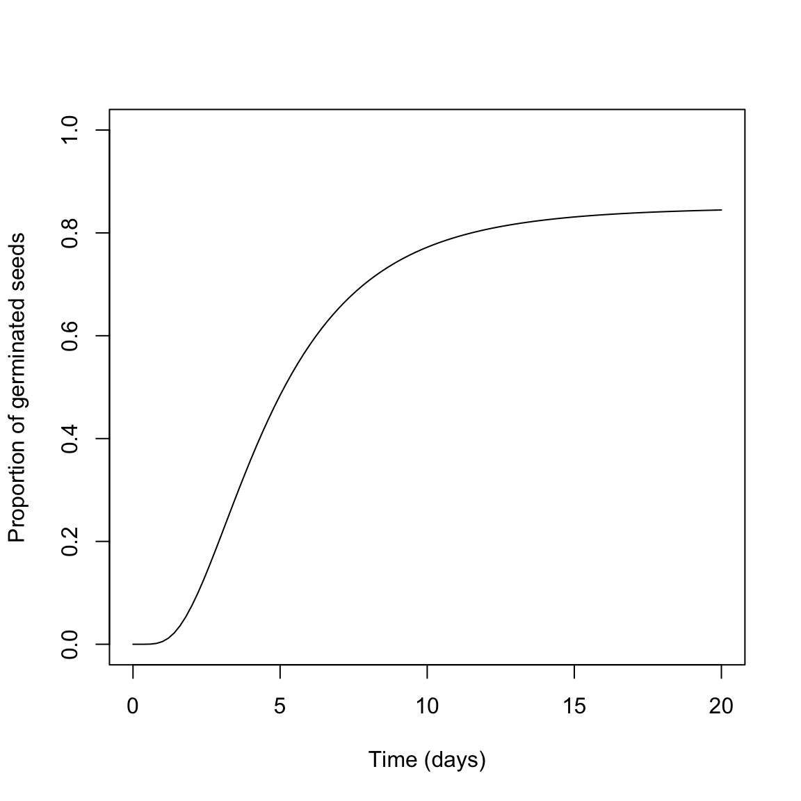
Usually, \(\Phi\) is right-skewed and, therefore, log-normal, log-logistic or Weibull cumulative distribution functions have been succesfully used. The graph below represents the germination time-course for a seed population with lognormal distribution of germination times, \(e = 4.5\) days, \(b = 0.6\) and a maximum germinated proportion \(d = 0.85\).
With log-normal or log-logistic distribution, \(e\) corresponds to the time to 50% germination (for the germinated fraction), while \(b\) relates to the standard deviation of germination times on a log-scale. Therefore, the three parameters of the germination curve have a clear biological meaning and they can be related to the three main features of seed germination, that is capability (\(d\)), uniformity (\(b\)) and speed (\(e\))
Germination assays are most often organised to be able to determine the germination curve for a given seed lot. In this tutorial, we will see that this may not be an easy task, as several statistical problems may arise during the process of model fitting. In particular, we have to deal with the problem of censoring, or else known as ‘grouped data’. If you would like to know more about this, please go to the following page.