Chapter 7 One-way ANOVA models

To find out what happens when you change something, it is necessary to change it (Box, Hunter and Hunter)

In Chapter 4 we have seen that the experimental observations can be described by way of models with both a deterministic and a stochastic component. With specific reference to the former component, we have already introduced an example of an ANOVA model, belonging to a very important class of linear models, where the response variable is quantitative, while the predictors are represented by one or several nominal explanatory factors. It is necessary to state that, strictly speaking, the term ‘ANOVA model’ is slightly imprecise; indeed, ANOVA stands for ANalysis Of VAriance and it is a method for decomposing the variance of a group of observations, which was invented by Ronald Fisher, almost one century ago. However, the models we are discussing here are strongly connected to the Fisherian ANOVA, which motivates their name.

In this Chapter we will use a simple (but realistic) example to introduce the ANOVA models with only one predictor (one-way ANOVA models).

7.1 Comparing herbicides in a pot-experiment

We have designed a pot-experiment to compare weed control efficacy of two herbicides used alone and in mixture. A control was also added as a reference and, thus, the four treatments were:

Metribuzin
Rimsulfuron
Metribuzin + rimsulfuron
Untreated control

Sixteen uniform pots were prepared and sown with Solanum nigrum; when the plants were at the stage of 4-true-leaves, the pots were randomly sprayed with the above herbicide solution, according to a completely randomised design with four replicates. Three weeks after the treatment, the plants in each pot were harvested and weighted: the lower the weight the higher the efficacy of herbicides.

The results of this experiment are reported in a ‘csv’ file, that is available in a web repository. First of all, let’s load the data into R.

repo <- "https://www.casaonofri.it/_datasets/"
file <- "mixture.csv"
pathData <- paste(repo, file, sep = "")

dataset <- read.csv(pathData, header = T)
head(dataset)
##             Treat Weight
## 1 Metribuzin__348  15.20
## 2 Metribuzin__348   4.38
## 3 Metribuzin__348  10.32
## 4 Metribuzin__348   6.80
## 5     Mixture_378   6.14
## 6     Mixture_378   1.95

Please, note that the dataset is in a ‘tidy’ format, with one row per observation and one column per variable. The first row contains the names of variables. i.e., ‘Treat’, representing the factor level and ‘Weight’, representing the response variable. While other data formats might be more suitable for visualisation, the ‘tidy’ format is the base of every statistical analyses with most software tools and it can be easily transformed into other formats, whenever necessary (Wichkam, 2014).

7.2 Data description

The first step is the description of the observed data. In particular, we calculate:

sample means for each treatment level
sample standard deviations for each treatment level

To do so, we use the tapply() function, as shown in the box below and we also use the data.frame() function to create a data table for visualisation purposes.

treatMeans <- tapply(dataset$Weight, dataset$Treat, mean)
SDs <- tapply(dataset$Weight, dataset$Treat, sd)
descrit <- data.frame(treatMeans, SDs)
descrit
##                 treatMeans      SDs
## Metribuzin__348     9.1750 4.699089
## Mixture_378         5.1275 2.288557
## Rimsulfuron_30     16.8600 4.902353
## Unweeded           26.7725 3.168673

What do we learn, from the above table of means? We learn that:

the mixture is slightly more effective than the herbicides used alone;
the standard deviations are rather similar, for all treatments.

Now, we ask ourselves: is there any significant difference between the efficacy of herbicides? If we look at the data, the answer is yes; indeed, the four means are different. However, we do not want to reach conclusions about our dataset; we want to reach general conclusions. We observed the four means $m_1$, $m_2$, $m_3$ and $m_4$, but we are interested in $\mu_1$, $\mu_2$, $\mu_3$ and $\mu_4$, i.e. the means of the populations from where our samples were drawn. What are the populations, in this case? They consist of all possible pots that we could have treated with each herbicide, in our same environmental conditions.

7.3 Model definition

In order to answer the above question, we need to define a suitable model to describe our dataset. A possible candidate model is:

\[Y_i = \mu + \alpha_j + \varepsilon_i\]

This model postulates that each observation $Y_i$ derives from the value $\mu$ (so called intercept and common to all observations) plus the amount $\alpha_j$, that depends on the treatment group $j$, plus the stochastic effect $\varepsilon_i$, which is specific to each observation and represents the experimental error. This stochastic element is regarded as gaussian distributed, with mean equal to 0 and standard deviation equal to $\sigma$. In mathematical terms:

\[\varepsilon_i \sim N(0, \sigma)\]

The expected value for each observation, depending on the treatment group, is

\[\bar{Y_i} = \mu + \alpha_j = \mu_j\]

and corresponds to the group mean. In order to understand the biological meaning of $\mu$ and $\alpha$ values we need to go a little bit more into the mathematical detail.

7.3.1 Parameterisation

Let’s consider the first observation $Y_1 = 15.20$; we need to estimate three values ($\mu$, $\alpha_1$ and $\varepsilon_1$) which return 15.20, by summation. Clearly, there is an infinite number of such triplets and, therefore, the estimation problem is undetermined, unless we put constraints on some model parameters. There are several ways to put such constraints, corresponding to different model parameterisations; in the following section, we will list two of them: the treatment constraint and the sum-to-zero constraint.

7.3.2 Treatment constraint

A very common constraint is $\alpha_1 = 0$. As the consequence:

\[\left\{ {\begin{array}{l} \mu_1 = \mu + \alpha_1 = \mu + 0\\ \mu_2 = \mu + \alpha_2 \\ \mu_3 = \mu + \alpha_3 \\ \mu_4 = \mu + \alpha_4 \end{array}} \right.\]

With such a constraint, $\mu$ is the mean for the first treatment level (in R, it is the first in alphabetical order), while $\alpha_2$, $\alpha_3$ and $\alpha_4$ are the differences between, respectively, the second, third and fourth treatment level means, with respect to the first one.

In general, with this parameterisation, model parameters are means or differences between means.

7.3.3 Sum-to-zero constraint

Another possible constraint is $\sum{\alpha_j} = 0$. If we take the previous equation and sum all members we get:

\[\mu_1 + \mu_2 + \mu_3 + \mu_4 = 4 \mu + \sum{\alpha_j}\]

Imposing the sum-to-zero constraint we get to:

\[\mu_1 + \mu_2 + \mu_3 + \mu_4 = 4 \mu\]

and then to:

\[\mu = \frac{\mu_1 + \mu_2 + \mu_3 + \mu_4}{4}\]

Therefore, with this parameterisation $\mu$ is the overall mean, while the $\alpha_j$ values represent the differences between each treatment mean and the overall mean (treatment effects). A very effective herbicide will have low negative $\alpha$ values, while a bad herbicide will have high positive $\alpha$ values.

In general, with this parameterisation, model parameters represent the overall mean and the effects of the different treatments.

The selection of constraints is up to the user, depending on the aims of the experiment. In this book, we will use the sum-to-zero constraint for our hand-calculations, as parameter estimates are easier to obtain and have a clearer biological meaning. In R, the treatment constraint is used by default, although the sum-to-zero constraint can be easily obtained, by using the appropriate coding. Independent on model parameterisation, the expected values, the residuals and all the other statistics are totally equal.

7.4 Basic assumptions

The ANOVA model above makes a number of basic assumptions:

the effects are purely additive;
there are no other effects apart from the treatment and random noise. In particular, there are no components of systematic error;
errors are independently sampled from a gaussian distribution;
error variances are homogeneous, independent from the experimental treatments (indeed, we only have one $\sigma$ value, common to all treatment groups)

We need to always make sure that the above assumptions are tenable, otherwise our model will be invalid, as well as all inferences therein. We will discuss this aspect in the next chapter.

7.5 Fitting ANOVA models by hand

Model fitting is the process by which we take the general model defined above and use the data to find the most appropriate values for the unknown parameters. In general, linear models are fitted by using the least squares approach, i.e. we look for the parameter values that minimise the squared difference between the observed data and model predictions. Nowadays, such minimisation is always carried out by using a computer, although we think that, once in life, fitting ANOVA models by hand may be very helpful, to understand the fundamental meaning of such a brilliant technique. In order to ease the process, we will not use the least squares method, but we will use the arithmetic means and the method of moments. Please, remember that this method is only appropriate when the data are balanced, i.e. when the number of replicates is the same for all treatment groups.

7.5.1 Parameter estimation

According to the sum-to-zero constraint, we calculate the overall mean (m) as:

m <- mean(dataset$Weight)
mu <- m

and our point estimate is $\mu = m = 14.48375$. Next, we can estimate the $\alpha$ effects by subtracting the overall mean from the group means:

alpha <- treatMeans - mu
alpha
## Metribuzin__348     Mixture_378  Rimsulfuron_30        Unweeded 
##        -5.30875        -9.35625         2.37625        12.28875

Please, note that the last parameter $\alpha_4$ was not ‘freely’ selected, as it was implicitly constrained to be:

\[\alpha_4 = - \left( \alpha_1 + \alpha_2 + \alpha_3 \right)\]

Now, to proceed with our hand-calculations, we need to repeat each $\alpha$ value four times, so that each original observation is matched to the correct $\alpha$ value, depending on the treatment group (see later).

alpha <- rep(alpha, each = 4)

7.5.2 Residuals

After deriving $\mu$ and $\alpha$ values, we can calculate the expected values by using the equation above and, lately, the residuals, as:

\[ \varepsilon_i = Y_i - \left( \mu - \alpha_j \right)\]

The results are shown in the following prospect:

Expected <- mu + alpha
Residuals <- dataset$Weight - Expected
tab <- data.frame(dataset$Treat, dataset$Weight, mu,
             alpha, Expected, Residuals)
names(tab)[1] <- "Herbicide"
print(tab, digits = 3)
##          Herbicide dataset.Weight   mu alpha Expected Residuals
## 1  Metribuzin__348          15.20 14.5 -5.31     9.18    6.0250
## 2  Metribuzin__348           4.38 14.5 -5.31     9.18   -4.7950
## 3  Metribuzin__348          10.32 14.5 -5.31     9.18    1.1450
## 4  Metribuzin__348           6.80 14.5 -5.31     9.18   -2.3750
## 5      Mixture_378           6.14 14.5 -9.36     5.13    1.0125
## 6      Mixture_378           1.95 14.5 -9.36     5.13   -3.1775
## 7      Mixture_378           7.27 14.5 -9.36     5.13    2.1425
## 8      Mixture_378           5.15 14.5 -9.36     5.13    0.0225
## 9   Rimsulfuron_30          10.50 14.5  2.38    16.86   -6.3600
## 10  Rimsulfuron_30          20.70 14.5  2.38    16.86    3.8400
## 11  Rimsulfuron_30          20.74 14.5  2.38    16.86    3.8800
## 12  Rimsulfuron_30          15.50 14.5  2.38    16.86   -1.3600
## 13        Unweeded          24.62 14.5 12.29    26.77   -2.1525
## 14        Unweeded          30.94 14.5 12.29    26.77    4.1675
## 15        Unweeded          24.02 14.5 12.29    26.77   -2.7525
## 16        Unweeded          27.51 14.5 12.29    26.77    0.7375

7.5.3 Standard deviation $\sigma$

In order to get an estimate for $\sigma$, we calculate the Residual Sum of Squares (RSS):

RSS <- sum(Residuals^2)
RSS
## [1] 184.1774

In order to obtain the residual variance, we need to divide the RSS by the appropriate number of Degrees of Freedom (DF); the question is: what is this number? We need to consider that the residuals represent the differences between each observed value and the group mean; therefore, those residuals must sum up to zero within all treatment groups, so that we have 16 residuals, but only three per group are ‘freely’ selected, while the fourth one must be equal to the opposite of the sum of the other three. Hence, the number of degrees of freedom is $3 \times 4 = 12$.

In more general terms, the number of degrees of freedom for the RSS is $p (k -1)$, where $p$ is the number of treatments and $k$ is the number of replicates (assuming that this number is constant across treatments). The residual variance is:

\[MS_{e} = \frac{184.178}{12} = 15.348\]

Consequently, our best point estimate for $\sigma$ is:

\[sigma = \sqrt{15.348} = 3.9177\]

Now, we can use our point estimates for model parameters to calculate point estimates for the group means (e.g.: $\mu_1 = \mu + \alpha_1$), which, in this instance, are equal to the arithmetic means, although this is not generally true. However, we know that point estimates are not sufficient to draw general conclusions and we need to provide the appropriate confidence intervals.

7.5.4 SEM and SED

The standard errors for the four means are easily obtained, by the usual rule ($k$ is the number of replicates):

\[SEM = \frac{s}{ \sqrt{k}} = \frac{3.918}{ \sqrt{4}}\]

You may have noted that, for all experiments, there are two ways to calculate standard errors for the group means:

by taking the standard deviations for each treatment group, as shown in Chapter 3. With $k$ treatments, this method results in $k$ different standard errors;
by taking the pooled standard deviation estimate $s$. In this case, we have only one common SEM value, for all group means.

You may wonder which method is the best. Indeed, if the basic assumption of variance homogeneity is tenable, the second method is better, as the pooled SEM is estimated with higher precision, with respect to the SEs for each group mean (12 degrees of freedom, instead of 3).

The standard error for the difference between any possible pairs of means is:

\[SED = \sqrt{ MS_{1} + MS_{2} } = \sqrt{ 2 \cdot \frac{MS_e}{n} } = \sqrt{2} \cdot \frac{3.9177}{\sqrt{4}} = \sqrt{2} \cdot SEM\]

7.5.5 Variance partitioning

Fitting the above model is prodromic to the Fisherian ANalysis Of VAriance, i.e. the real ANOVA technique. The aim is to partition the total variability of all observations into two components: the first one is due to treatment effects and the other one is due to all other effects of random nature.

In practice, we start our hand calculations from the total sum of squares (SS), that is the squared sum of residuals for each value against the overall mean (see Chapter 3):

\[\begin{array}{c} SS = \left(24.62 - 14.48375\right)^2 + \left(30.94 - 14.48375\right)^2 + ... \\ ... + \left(15.50 - 14.48375\right)^2 = 1273.706 \end{array}\]

Total deviance relates to the all the effects, both from known and unknown sources (treatment + random effects). With R:

SS <- sum( (dataset$Weight - mu)^2 )

Second, we can consider that the RSS represents the amount of data variability produced by random effects. Indeed, the variability of data within each treatment group cannot be due to treatment effects.

Finally, we can consider that variability produced by treatment effects is measured by the $\alpha$ values and, therefore, the treatment sum of squares (TSS) is given by the sum of squared $\alpha$ values:

TSS <- sum(tab$alpha^2)
TSS
## [1] 1089.529

Please, note that the sum of the residual sum of squares (RSS) and the treatment sum of squares (TSS) is exactly equal to the total sum of squares:

TSS + RSS
## [1] 1273.706

The partitioning of total variance shows that random variability is much lower than treatment variability, although we know that we cannot directly compare two deviances, when they are based on a different number of DFs (see Chapter 3).

Therefore, we calculate the corresponding variances: we have seen that the RSS has 12 degrees of freedom and the related variance is $MS_e = 15.348$. The TSS has 3 degrees of freedom, that is the number of treatment levels minus one; the related variance is:

\[MS_t = \frac{1089.529}{3} = 363.1762\]

These two variances (treatment and residual) can be directly compared. Fisher, in 1920, proposed the following F-ratio:

\[F = \frac{MS_t}{MS_e} = \frac{363.18}{15.348} = 23.663\]

It shows that the variability imposed by the experimental treatment is more than 23 times higher than the variability due to random noise, which supports the idea that the treatment effect is significant. However, we need a formal statistical test to support such a statement.

7.5.6 Hypothesis testing

Let me recall a basic concept that has already appeared before and it is going to return rather often in this book (apologies for this). We have observed a set of 16 data, coming from a pot-experiment, but these data represent only a sample of an infinite number of replicated experiments that we could perform. Therefore, the observed F value is just an instance of an infinite number of possible F values, which define a sampling distribution. How does such sampling distribution look like?

In order to determine the sampling distribution for the F-ratio, we need to make some hypotheses. The null hypothesis is that the treatments have no effects and, thus:

\[H_0: \mu_1 = \mu_2 = \mu_3 = \mu_4\]

Analogously:

\[H_0: \alpha_1 = \alpha_2 = \alpha_3 = \alpha_4 = 0\]

In other words, if $H_0$ were true, the four samples would be drawn from the same gaussian population. What would become of the F-ratio? We could see this by using Monte Carlo simulation, but, for the sake of simplicity, let’s exploit literature information: the American mathematician George Snedecor demonstrated that, when the null is true, the sample based F-ratio is distributed according to the F-distribution (Fisher-Snedecor distribution). In more detail, Snedecor defined a family of F-distributions, whose elements are selected, depending on the number of degrees of freedom at the numerator and denominator. For our example (three degrees of freedom at the numerator and 12 at the denominator), the F distribution is shown in Figure 7.1. We see that the mode is between 0 and 1, while the expected value is around 1. We also see that values above 6 are very unlikely.

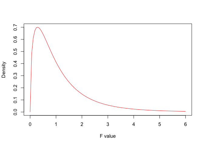
Figure 7.1: Probabilty density function for F distribution with three and twelve degrees of freedom

Now, we can use the cumulative distribution function in R to calculate the probability of obtaining values as high as 23.663 (the observed value) or higher:

pf(23.663, 3, 12, lower.tail = F)
## [1] 2.508789e-05

We can see that, if the hull is true and we repeat the experiment a very high humber of times, there is only one chance in 250,000 that we observe such a high F-value. As the consequence, we reject the null and accept the alternative, i.e. there is at least one treatment level that produced a significant effect.

7.6 Fitting ANOVA models with R

Fitting models with R is very straightforward, by way of a very consistent platform for most types of models. For linear models, we use the lm() function, according to the following syntax:

mod <- lm(Weight ~ factor(Treat), data = dataset)

The first argument is the equation we want to fit: on the left side, we specified the name of the response variable, the ‘tilde’ means ‘is a function of and replaces the = sign and, on the right side, we specified the name of the factor variable. We did not specify the intercept and the stochastic term $\varepsilon$, which are included by default. Please, also note that, prior to analysis, we transformed the ’Treat’ variable into a factor, by using the factor() function. Such a transformation is not strictly necessary with character variables, but becomes fundamental with numeric variables, representing numbers and not classes.

dataset$Treat <- factor(dataset$Treat)
mod <- lm(Weight ~ Treat, data = dataset)

After fitting the model, results are written into the ‘mod’ variable and can be read by using the appropriate extractor ($ sign) or by using some of the available methods. For example, the summary() method returns parameter estimates, according to the treatment constraint, that is the default in R.

summary(mod)
## 
## Call:
## lm(formula = Weight ~ Treat, data = dataset)
## 
## Residuals:
##    Min     1Q Median     3Q    Max 
## -6.360 -2.469  0.380  2.567  6.025 
## 
## Coefficients:
##                     Estimate Std. Error t value Pr(>|t|)    
## (Intercept)            9.175      1.959   4.684 0.000529 ***
## TreatMixture_378      -4.047      2.770  -1.461 0.169679    
## TreatRimsulfuron_30    7.685      2.770   2.774 0.016832 *  
## TreatUnweeded         17.598      2.770   6.352 3.65e-05 ***
## ---
## Signif. codes:  0 '***' 0.001 '**' 0.01 '*' 0.05 '.' 0.1 ' ' 1
## 
## Residual standard error: 3.918 on 12 degrees of freedom
## Multiple R-squared:  0.8554, Adjusted R-squared:  0.8193 
## F-statistic: 23.66 on 3 and 12 DF,  p-value: 2.509e-05

For the sake of completeness, it might be useful to show that we can change the parameterisation, by setting the argument ‘contrasts’ and passing a list of factors associated to the requested parameterisation (Treat = “contr.sum”, in this case). There are other methods to change the parameterisation, either globally (for the whole R session) or at the factor level; further information can be found in literature.

mod2 <- lm(Weight ~ Treat, data = dataset,
           contrasts = list(Treat = "contr.sum"))
summary(mod2)$coef
##             Estimate Std. Error   t value     Pr(>|t|)
## (Intercept) 14.48375  0.9794169 14.788135 4.572468e-09
## Treat1      -5.30875  1.6963999 -3.129421 8.701206e-03
## Treat2      -9.35625  1.6963999 -5.515356 1.329420e-04
## Treat3       2.37625  1.6963999  1.400761 1.866108e-01

Regardless of the parameterisation, fitted values and residuals can be obtained by using the fitted() and residuals() methods:

expected <- fitted(mod)
epsilon <- residuals(mod)

The residual deviance is:

deviance(mod)
## [1] 184.1774

while the residual standard deviation needs to be extracted from the slot ‘sigma’, from the output of the summary() method:

summary(mod)$sigma
## [1] 3.917668

The ANOVA table is obtained by using the anova() method:

anova(mod)
## Analysis of Variance Table
## 
## Response: Weight
##           Df  Sum Sq Mean Sq F value    Pr(>F)    
## Treat      3 1089.53  363.18  23.663 2.509e-05 ***
## Residuals 12  184.18   15.35                      
## ---
## Signif. codes:  0 '***' 0.001 '**' 0.01 '*' 0.05 '.' 0.1 ' ' 1

7.7 Expected marginal means

At the beginning of this chapter we have used the arithmetic means to describe the central tendency of each group. We have also seen that the sums $\mu + \alpha_j$ return the group means, taking the name Expected Marginal Means (EMMs), which can also be used as measures of central tendency. When the experiment is balanced (same number of replicates for all groups), EMMs are equal to the arithmetic means, while, when the experiment is unbalanced, they differ and provide better estimators of population means.

In order to obtain expected marginal means with R, we need to install the add-in package ‘emmeans’ (Lenth, 2016) and use the emmeans() function therein.

# Install the package (only at the very first instance)
# install.packages("emmeans") 
library(emmeans) # Load the package
muj <- emmeans(mod, ~Treat)
muj
##  Treat           emmean   SE df lower.CL upper.CL
##  Metribuzin__348   9.18 1.96 12     4.91     13.4
##  Mixture_378       5.13 1.96 12     0.86      9.4
##  Rimsulfuron_30   16.86 1.96 12    12.59     21.1
##  Unweeded         26.77 1.96 12    22.50     31.0
## 
## Confidence level used: 0.95

7.8 Conclusions

Fitting ANOVA models is the subject of several chapters in this book. In practice, we are interested in assessing whether the effect of treatments produces a bigger data variability than all other unknown stochastic effects. We do so by using the F ratio that, under the null hypothesis, has a Fisher-Snedecor F distribution. If the observed F value and higher values are very unlikely to occur under the null, we reject it and conclude that the treatment effect was significant.

Finally, it is very important to point out that all the above reasoning is only valid when the basic assumptions for linear models are met. Therefore, it is always important to make the necessary inspections to ensure that there are no evident deviations, as we will see in the next chapter.

7.9 Further readings

Faraway, J.J., 2002. Practical regression and Anova using R. http://cran.r-project.org/doc/contrib/Faraway-PRA.pdf.
Fisher, Ronald (1918). “Studies in Crop Variation. I. An examination of the yield of dressed grain from Broadbalk” (PDF). Journal of Agricultural Science. 11 (2): 107–135.
Kuehl, R. O., 2000. Design of experiments: statistical principles of research design and analysis. Duxbury Press (CHAPTER 2)
Lenth, R.V., 2016. Least-Squares Means: The R Package lsmeans. Journal of Statistical Software 69. https://doi.org/10.18637/jss.v069.i01
Wickham, H (2014) Tidy Data. J Stat Soft 59

Experimental methods in agriculture