Chapter 4 Modeling the experimental data
Models are wrong, but some are useful (G. Box)
In the previous chapter we have seen that we can use simple stats to describe, summarise and present our experimental data, which is usually the very first step of data analyses. However, we are more ambitious: we want to model our experimental data. Perhaps this term sounds unfamiliar to some of you and, therefore, we should better start by defining the terms ‘model’ and ‘modeling’.
A mathematical model is the description of a system using the mathematical language and the process of developing a model is named mathematical modeling. In practice, we want to write an equation where our experimental observations are obtained as the result of a set of predictors and operators.
Writing mathematical models for natural processes has been one of the greatest scientific challenges, since the 19th century and it may be appropriately introduced by using a very famous quote from Pierre-Simon Laplace (1749-1827): “We ought to regard the present state of the universe as the effect of its antecedent state and as the cause of the state that is to follow. An intelligence knowing all the forces acting in nature at a given instant, as well as the momentary positions of all things in the universe, would be able to comprehend in one single formula the motions of the largest bodies as well as the lightest atoms in the world, provided that its intellect were sufficiently powerful to subject all data to analysis; to it nothing would be uncertain, the future as well as the past would be present to its eyes. The perfection that the human mind has been able to give to astronomy affords but a feeble outline of such an intelligence.”
Working in biology and agriculture, we need to recognise that we are very far away from Laplace’s ambition; indeed, the systems which we work with are very complex and they are under the influence of a high number of external forces in strong interaction with one another. The truth is that we know too little to be able to predict the future state of the agricultural systems; think about the yield of a certain wheat genotype: in spite of our research effort, we are not yet able to forecast future yield levels, because, e.g., we are not yet able to forecast the weather for future seasons.
In this book, we will not try to write models to predict future outcomes for very complex systems; we will only write simple models to describe the responses obtained from controlled experiments, where the number of external forces has been reduced to a minimum level. You might say that modeling the past is rather a humble aim, but we argue that this is challenging enough…
One first problem we have to solve is that our experimental observations are always affected by:
- deterministic effects, working under a cause-effect relationship;
- stochastic effects, of purely random nature, which induce more or less visible differences among the replicates of the same measurement.
Clearly, every good descriptive model should contain two components, one for each of the above mentioned groups of effects. Models containing a random component are usually named ‘statistical models’, as opposed to ‘mathematical models’, which tend to disregard the stochastic effects.
4.1 Deterministic models
Based on the Galileian scientific approach, our hypothesis is that all biological phoenomena are based on an underlying mechanism, which we describe by using a deterministic (cause-effect) model, where:
\[ Y_E = f(X, \theta) \]
In words, the expected outcome \(Y_E\) is obtained as a result of the stimulus \(X\), according to the function \(f\), based on a number of parameters \(\theta\); this simple cause-effect model, with loose language, can be called a dose-response model.
Let’s look at model components in more detail. In a previous chapter we have seen that the expected response \(Y_E\) can take several forms, i.e. it can be either a quantity, or a count, or a ratio or a quality. The expected response can be represented by one single variable (univariate response) or by several variables (multivariate response) and, in this book, we will only consider the simplest situation (univariate response).
The experimental stimulus (\(X\)) is represented by one or more quantitative/categorical variables, usually called predictors, while the response function \(f\) is a linear/non-linear equation, that is usually selected according to the biological mechanism of the process under investigation. Very often, equations are selected in a purely empirical fashion: we look at the data and select a suitable curve shape.
Every equation is based on a number of parameters, which are generally indicated by using Greek or Latin letters. In this book we will use \(\theta\) to refer to the whole set of parameters in a deterministic model.
Let’s see a few examples of deterministic models. The simplest model is the so-called model of the mean, that is expressed as:
\[ Y = \mu \]
According to this simple model, the observations should be equal to some pre-determined value (\(\mu\)); \(f\) is the identity function with only one parameter (\(\theta = \mu\)) and no predictors. In this case, we do not need predictors, as the experiment is not comparative, but, simply, mensurative. For a comparative experiment, where we have two or more stimula, the previous model can be expanded as follows:
\[ Y = \left\{ {\begin{array}{ll} \mu_A \quad \textrm{if} \,\, X = A \\ \mu_B \quad \textrm{if} \,\, X = B \end{array}} \right. \]
This is a simple example of the so-called ANOVA models, where the response depends on the stimulus and subjects treated with A return a response equal to \(\mu_A\), while subjects treated with B return a response equal to \(\mu_B\). The response is quantitative, but the predictor represents the experimental treatments and it is described by using a categorical variable, with two levels. We can make it more general by writing:
\[Y = \mu_j\]
where \(j\) represents the experimental treatment.
Another important example is the simple linear regression model, where the relationship between the predictor and the response is described by using a ‘straight line’:
\[ Y = \beta_0 + \beta_1 \times X \]
In this case, both \(Y\) and \(X\) are quantitative variables and we have two parameters, i.e. \(\theta = [\beta_0, \beta_1]\).
We can also describe curvilinear relationships by using other models, such as a second order polynomial (three parameters):
\[ Y = \beta_0 + \beta_1 \, X + \beta_2 \, X^2\]
or the exponential function (two parameters, \(e\) is the Nepero operator):
\[ Y = \beta_0 \, e^{\beta_1 X} \]
We will see some more examples of curvilinear functions near to the end of this book.
Whatever it is, the function \(f\) needs to be fully specified, i.e. we need to give a value to all unknown parameters. Consider the following situation: we have a well that is polluted by herbicide residues to a concentration of 120 mg/L. If we analyse a water sample from that well, we should expect that the concentration is \(Y_E = 120\) (model of the mean). Likewise, if we have two genotypes (A and B), their yield in a certain pedo-climatic condition could be described by an ANOVA model, where we specify that, e.g.,
\[ Y = \left\{ {\begin{array}{ll} 27 \quad \textrm{if} \,\, X = A \\ 32 \quad \textrm{if} \,\, X = B \end{array}} \right. \]
As a third example of a fully specified model, we could assume that the yield response of wheat in some specific environmental conditions is related to N fertilisation, by way of a linear function \(Y = \beta_0 + \beta_1 \times X\), where \(\beta_0 = 20\) e \(\beta_1 = 0.3\) (i.e. \(\theta = [20, 0.3]\)). In this case, the model is \(Y = 20 + 0.3 \times X\) and we can use it to predict the yield response to, e.g., 0, 30, 60, 90, 120 and 150 kg N ha-1, as shown below:
You may argue that this latter example is not realistic, as the relationship between N fertilisation and yield can never be linear, but, presumably, asymptotic. You are right, but that does not matter at this moment; our point is that we can postulate the existence of an underlying, unknown mechanism that produces our experimental outcomes, by following a fully specified deterministic cause-effect model.
4.2 Stochastic models
In practice, reality is more complex than our expectations and, due to experimental errors, we do never observe the expected outcome. Therefore, modelling the observations requires that we introduce the effect of unknown entities. It would seem a nonsense… how can we predict the effects of something we do not even know?
Let’s go back to the example of the polluted well, where we would expect that the concentration is \(Y_E = 120\) mg/L. It is very easy to imagine that the above mechanism is overly simplistic, due to the fact that our chemical instrument is not free from measurement errors. Indeed, if we measure the concentration of several water samples from the same well, we will not always obtain exactly 120 mg/L, but we will obtain a set of values more or less different from each other. We could model this by writing that the observed values \(Y_O \neq Y_E\) is:
\[Y_O = 120 + \varepsilon\]
where \(\varepsilon\) is an individual random component that brings our measure away from the expected value. Do we have any hints on how to determine \(\varepsilon\)? If we had enough knowledge to understand the exact cause for the effect \(\varepsilon\) we could incorporate it into the deterministic model. As we do not have enough knowledge at the moment, we need to find another way to model this stochastic component.
Indeed, although we cannot precisely determine \(\varepsilon\) for each single water sample, we can make some reasonable assumptions. If the expected value is 120 mg/L (this is indeed the underlying mechanism we postulate), we should expect that it is likely to find a cooncentration of 119 or 121 mg/L (\(\varepsilon = \pm 1\)), less likely to find a concentration of 100 or 140 mg/L (\(\varepsilon = \pm 20\)), very unlikely to find a concentration of 80 or 160 mg/L (\(\varepsilon = \pm 40\)). Consequently, it should be possible to assign a value of probability to each possible \(\varepsilon\) value (and thus to each possible \(Y_O\) value), by using some sort of probability function.
4.2.1 Probability functions
How do we assign the probability to a stochastic experimental outcome? This is rather easy when the outcome \(Y_O\) is categorical and can only take one of a finite list of possible values \(y\). For example, let’s consider an experiment where we sample a wheat plant from a population and count the number of lateral tillers, so that \(Y_O\) can only take an integer value from, e.g., 0 to 3. The probability of finding a plant with, e.g., one lateral tiller (\(Y_O\) = 1) is equal to the number of subjects with one lateral tiller divided by the total number of subjects within the population (frequentist definition of probability). If the population consists of 20 plants and, among those, 4 plants have no lateral tillers, 6 plants have one tiller, 8 plants have 2 tillers and 2 plants have three tillers, the probabilities for all the possible outcomes are:
\[P(Y_O = y) = \left\{ \begin{array}{l} 4/20 = 0.2 \,\,\,\,\,\,\textrm{if}\,\,\,\,\,\, y = 0 \\ 6/20 = 0.3 \,\,\,\,\,\,\textrm{if}\,\,\,\,\,\, y = 1 \\ 8/20 = 0.4\,\,\,\,\,\, \textrm{if}\,\,\,\,\,\, y = 2 \\ 2/20 = 0.1 \,\,\,\,\,\,\textrm{if}\,\,\,\,\,\, y = 3 \\ \end{array} \right.\]
In the above equation, P is a Probability Mass Function (PMF) or, more simply a Probability Function and it takes the form of a distribution of relative frequencies. It does not help us to predict the outcome of our sampling experiment, but it gives us an idea of what it is more likely to happen.
What are the main characteristics of a probability function? Two rules are fundamental:
- \(P(Y_O = y)\) must always be positive, for every possible \(y\) value;
- the probabilities for all possible events \(y\) must sum up to one, i.e. \(\sum{P \left(Y_O = y \right)} = 1\)
With ordinal classes (as in our example), we can also define the Cumulative Distribution Function (CDFs), as the sum of the probabilities of one event with all the ‘previous’ ones, i.e.:
\[P(Y_O \le y) = \sum_{y_k \le y}{P(Y_O = y_k)}\]
For our wheat tillers example, we have:
\[P(Y_O \le y) = \left\{ \begin{array}{l} 0.2\,\,\,\,\,\,\textrm{if}\,\,\,\,\,\, y \leq 0 \\ 0.5\,\,\,\,\,\,\textrm{if}\,\,\,\,\,\, y \leq 1 \\ 0.9\,\,\,\,\,\,\textrm{if}\,\,\,\,\,\, y \leq 2 \\ 1.0\,\,\,\,\,\,\textrm{if}\,\,\,\,\,\, y \leq 3 \\ \end{array} \right.\]
For these PDFs, using the information given in Chapter 3, we can calculate descriptive statistics, such as the mean (expected value) and the variance:
\[\mu = \sum{\left[ y_k \cdot P(Y_O = y_k ) \right]}\]
\[\sigma ^2 = \sum{ \left[ {\left( {y_k - \mu } \right)^2 \cdot P(Y_O = y_k)} \right]}\]
In our example, it is:
and:
sigma2 <- (0 - mu)^2 * 0.2 + (1 - mu)^2 * 0.3 + (2 - mu)^2 *
  0.3 + (3 - mu)^2 * 0.2
sigma2
## [1] 1.06
On average, our plants have 1.4 lateral tillers, with a variance of 1.06.
4.2.2 Density functions
For quantitative variables, the outcome may take any value within a certain interval. Is it sensible to ask what probability we have to measure a concentration value that is exactly, e.g., 120 mg/L (not 120.0000001 or 119.99999 mg/L)? We do understand that such a probability is infinitesimal. In general, we cannot calculate the probability of a ‘point-event’ for continuous variables.
We can think of dividing the concentration scale into a finite number of intervals, e.g. < 100 mg/L, from 100 to 110 mg/L, from 110 to 120 mg/L and so on (binning; we spoke about this in Chapter 3), so that all individuals in the population can be assigned to one and only one interval. It is intuitively clear that we can always calculate the probability of one interval as the ratio between the number of individuals in that interval and the total number of individuals in the population. However, a new problem arises when we try to define a probability function: how should we select the width of intervals?
A possible solution is that we calculate the so-called probability density, i.e. the ratio of the probability mass in one interval to the interval width. For example, if we have a probability mass of 0.3 in the interval between 110 to 130 \(mg/L\), the probability density is:
\[D([110, 130]) = \frac{P([110,130])}{20} = \frac{0.3}{20}\]
Why do we talk about ‘density’? Because this is, indeed, a probability mass per unit interval (do you remember? the usual density is a mass per unit volume).
Now we can wonder: what happens with the density, when the interval becomes smaller and smaller? This is shown in Figure 4.1; we can see that when the interval width tends to 0, the density tends to assume a finite value, according to the red function in Figure 4.1 (bottom right).
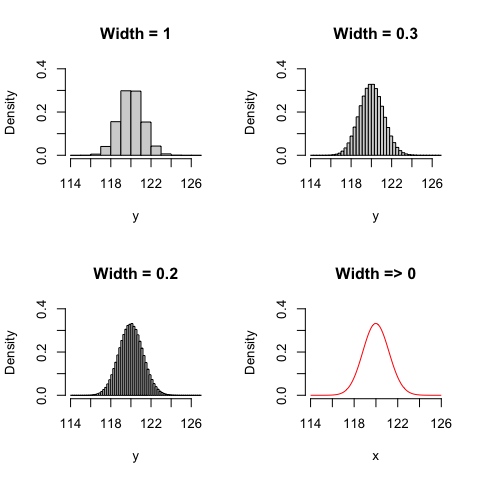
Figure 4.1: Probability density function, depending on the width of the interval
In the end, dealing with a continuous variable, we cannot calculate the probability of a ‘point-event’, but we can calculate its density. Therefore, instead of defining a probability function, we can define a Probability Density Function (PDF), depicting the density of all possible events.
The most common PDF is the Gaussian PDF, that is also known as the normal curve; it is represented in the bottom right panel of Figure 4.1 and it is introduced in the following section.
4.2.3 The Gaussian PDF and CDF
The Gaussian PDF is defined as:
\[\phi(y) = \frac{1}{{\sigma \sqrt {2\pi } }}\exp \left[{\frac{\left( {y - \mu } \right)^2 }{2\sigma ^2 }} \right]\]
where \(\phi(y)\) is the probability density that the observed outcome assume the value \(y\), while \(\mu\) and \(\sigma\) are the parameters. The gassian PDF is continuous and it is defined from \(-\infty\) to \(\infty\).
The density in itself is not very much useful for our task; how can we use the density to calculate the probability for an outcome \(Y_O\) that is comprised between any two values \(y_1\) and \(y_2\)?. Let’s recall that the density is the probability mass per unit interval width; therefore, if we multiply the density by the interval width, we get the probability for that interval. We can imagine that the area under the gaussian curve in Figure 4.1 (bottom right) is composed by a dense comb of tiny rectangles with very small widths; the area of each rectangle is obtained as the product of a density (height) by the interval width and, therefore, it represents a probability. Consequently, if we take any two values \(y_1\) and \(y_2\), the probability of the corresponding interval can be obtained as the sum of the areas of all the tiny rectangles between \(y_1\) and \(y_2\). In other words, the probability of an interval can be obtained as the Area Under the Curve (AUC). You may recall from high school that the AUC is, indeed, the integral of the gaussian curve from \(y_1\) and \(y_2\):
\[P(y_1 \le Y_O < y_2) = \int\limits_{ y_1 }^{y_2} {\phi(y)} dy\]
Analogously, we can obtain the corresponding CDF, by:
\[P(Y_O \le y) = \int\limits_{ -\infty }^{y} {f(y)} dy\]
You may have noted that this is totally the same as the PDF for a discrete variable, although the summation has become an integral.
If the PDF is the defined as the function \(\phi(y)\), the mean and variance for \(\phi\) can also be calculated as shown above for the probability functions, by replacing summations with integrals:
\[\begin{array}{l} \mu = \int\limits_{ - \infty }^{ + \infty } {y f(y)} dy \\ \sigma ^2 = \int\limits_{ - \infty }^{ + \infty } {\left( {y - \mu } \right)^2 f(y)} dy \end{array}\]
I will not go into much mathematical detail, but it is useful to note that, with a Gaussian CDF:
- the curve shape depends only on the values of \(\mu\) and \(\sigma\) (Figure 4.2 ). It means that if we start from the premise that a population of measures is Gaussian distributed (normally distributed), knowing the mean and the standard deviation is enough to characterise the whole population. Such a premise is usually called parametric assumption.
- The curve has two asymptotes and the limits when \(y\) goes to \(\pm \infty\) are 0. It is implied that every \(y\) values is a possible outcome for our experiment, although the probabilities of very small and very high values are negligible.
- The integral of the Gauss curve from \(- \infty\) to \(+ \infty\) is 1, as this is the sum of the probability densities for all possible outcomes.
- The area under the Gaussian curve between two points (integral) represents the probability of obtaining values within the corresponding interval. For example, Figure 4.3 shows that 80% of the individuals lie within the interval from \(-\infty\) to, roughly, 1;
- The curve is symmetrical around the mode, that is equal to the median and the mean. That is, the probability density of values above the mean and below the mean is equal.
- We can calculate that, for given \(\mu\) and \(\sigma\), the probability density of individuals within the interval from \(\mu\) to \(\mu + \sigma\) is 15.87% and it is equal to the probability density of the individuals within the interval from \(\mu - \sigma\) to \(\mu\).
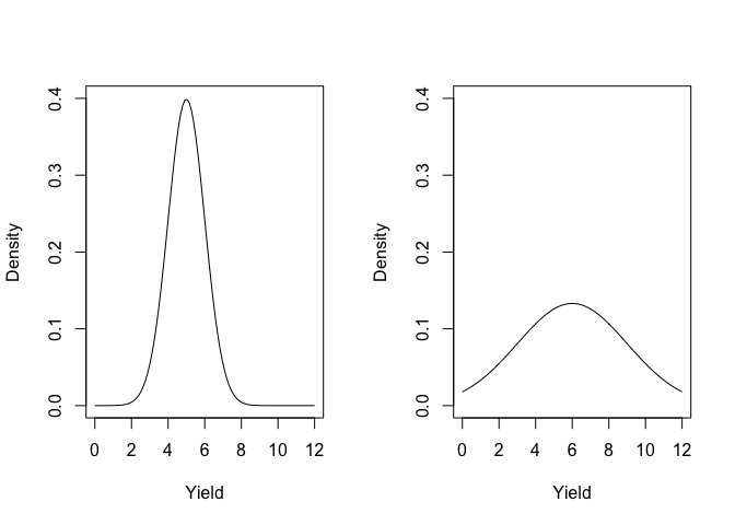
Figure 4.2: The shape of the gaussian function, depending on the mean and standard deviation (left: mean = 5 and SD = 1; right: mean = 6 and SD = 3)
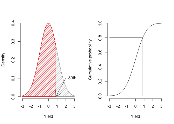
Figure 4.3: Getting the 80th percentile as the area under the PDF curve (left) and from the CDF (right)
4.3 A model with two components
Let’s go back to our example with the polluted well. We said that, on average, the measure should be 120 mg/L, but we also said that each individual measure has its own random component \(\epsilon\), so that \(Y_O = 120 + \varepsilon\). The stochastic element cannot be predicted, but we can use the Gaussian to calculate the probability of any outcome \(Y_O\).
Now we are ready to write a two-components model for our herbicide concentrations, in relation to each possible water sample \(i\):
\[y_i = \mu + \varepsilon_i\]
where the stochastic element \(\varepsilon\) is:
\[ \varepsilon \sim \textrm{Norm}(0, \sigma) \]
The above equation means that the stochastic element is gaussian distributed with mean equal to 0 and standard deviation equal to \(\sigma\). Another equivalent form is:
\[Y_i \sim \textrm{Norm}(\mu, \sigma)\]
which says that the concentration is gaussian distributed with mean \(\mu = 120\) (the deterministic part) and standard deviation equal to \(\sigma\).
In our example, if we assume that \(\sigma = 12\) (the stochastic part), we can give the best possible description of all concentration values for all possible water samples from our polluted well. For example, we can answer the following questions:
- What is the most likely concentration value?
- What is the probability density of finding a water sample with a concentration of 100 mg/L?
- What is the probability of finding a water sample with a concentration lower than 100 mg/L?
- What is the probability of finding a water sample with a concentration higher than 140 mg/L?
- What is the probability of finding a water sample with a concentration within the interval from 100 to 140 mg/L?
- What is the 80th percentile, i.e. the concentration which is higher than 80% of all possible water samples?
- What are the two values, symmetrical around the mean, which contain the concentrations of 95% of all possible water samples?
Question 1 is obvious. In order to answer all the above questions from 2 on, we need to use the available R function for gaussian distribution. For every distribution, we have a PDF (the prefix is always ‘d’), a CDF (the prefix is ‘p’) and a quantile function (the prefix is ‘q’), that is the inverse CDF, giving the value corresponding to a given percentile. For the Gaussian function, the name is ‘norm’, so that we have the R functions dnorm(), pnorm() and qnorm(). The use of these functions is straightforward:
For the 4th question we should consider that cumulative probabilities are given for the lower curve tail, while we were asked to determine the higher tail. Therefore, we have two possible solutions, as shown below:
# Question 4
1 - pnorm(140, mean = 120, sd = 12)
## [1] 0.04779035
pnorm(140, mean = 120, sd = 12, lower.tail = F)
## [1] 0.04779035In order to calculate the percentiles we use the qnorm() function:
4.4 And so what?
Let’s summarise:
- we use deterministic cause-effect models to predict the average behavior in a population
- we cannot predict the exact outcome of each single experiment, but we can calculate the probability of obtaining one of several possible outcomes by using stochastic models, in the form of PDFs
In order to do so, we need to be able to assume what the form is for the PDF within the population (parametric assumption). Indeed, such a form can only be assumed, unless we know the whole population, which is impossible as long as we are making an experiment to know the population itself.
4.5 Monte Carlo methods to simulate an experiment
Considering the above process, the results of every experiment can be simulated by using the so-called Monte Carlo methods, which can reproduce the mechanisms of natural phenomena. These methods are based on random number generators; for example, in R, it is possible to produce random numbers from a given PDF, by using several functions prefixed by ‘r’. For example, the gaussian random number generator is rnorm().
Let’s go back to our polluted well. If we know that the concentration is exactly 120 mg/L, we can reproduce the results of an experiment where we analyse three replicated water samples, by using an instrument with 10% coefficient of variability (that is \(\sigma = 12\)).
With R, the process is as follows:
set.seed(1234)
Y_E <- 120
epsilon <- rnorm(3, 0, 12)
Y_O <- Y_E + epsilon
Y_O
## [1] 105.5152 123.3292 133.0133
We need to note that, at the very beginning, we set the seed to the value of ‘1234’. Indeed, random numbers are, by definition, random and, therefore, we should all obtain different values at each run. However, random number generators are based on an initial ‘seed’ and, if you and I set the same seed, we can obtain the same random values, which is handy, for the sake of reproducibility. Please, also note that the first argument to the rnorm() function is the required number of random values.
The very same approach can be used with more complex experiments:
- simulate the expected results by using the selected deterministic model,
- attached random variability to the expected outcome, by sampling from the appropriate probability density function, usually by a gaussian.
In the box below we show how to simulate the results of an experiment where we compare the yield of wheat treated with four different nitrogen rates (0, 60, 120 e 180 kg/ha), on an experiment with four replicates (sixteen data in all).
set.seed(1234)
Dose <- rep(c(0, 60, 120, 180), each=4)
Yield_E <- 25 + 0.15 * Dose
epsilon <- rnorm(16, 0, 2.5)
Yield <- Yield_E + epsilon
dataset <- data.frame(Dose, Yield)
dataset
##    Dose    Yield
## 1     0 21.98234
## 2     0 25.69357
## 3     0 27.71110
## 4     0 19.13576
## 5    60 35.07281
## 6    60 35.26514
## 7    60 32.56315
## 8    60 32.63342
## 9   120 41.58887
## 10  120 40.77491
## 11  120 41.80702
## 12  120 40.50403
## 13  180 50.05937
## 14  180 52.16115
## 15  180 54.39874
## 16  180 51.72429
4.6 Data analysis and model fitting
So far, we have shown how we can model the outcome of scientific experiments. In practise, we have assumed that we knew the function \(f\), the parameters \(\theta\), the predictors \(X\) the PDF type and \(\sigma\). With such knowledge, we have produced the response \(y_i\). In an experimental setting the situation is the reverse: we know the predictors \(X\), the measured response \(y_i\) and we can assume a certain form for \(f\) and for the PDF, but we do not know \(\theta\) and \(\sigma\).
Therefore, we use the observed data to estimate \(\theta\) and \(\sigma\). We see that we are totally following the Galileian process, by posing our initial hypothesis in the form of a mathematical model. This process is named model fitting and we will see that, most of the times, analyzing the data can be considered as a process of model fitting. We will also see that once the unknown parameters have been retrieved from the data, we will have to assess whether the fitted model represents an accurate description of our data (model evaluation). Likewise, comparing different hypothesis about the data can be seen as a process of model comparison. Those are the tasks that will keep us busy in the following chapters.
4.7 Some words of warning
In this chapter we have only considered one stochastic model, that is the Gaussian PDF. Of course, this is not the only possibility and there are several other probability density functions which can be used to achieve the same aim, i.e. describing random variability. For example, in Chapter 5 we will see the Student’s t distribution and, in Chapter 7, we will see the Fisher-Snedecor distribution. For those who are interested further information about non-gaussian PDFs can easily be found in the existing literature (see the great Bolker’s book, that is cited below).