Chapter 5 Estimation of model parameters

Death is a fact. All else is inference (W. Farr)

In chapter 4 we have shown that the experimental data can be regarded as the outcome of a deterministic cause-effect process, where a given stimulus is expected to produce a well defined response. Unfortunately, the stochastic effects of experimental errors (random noise) ‘distort’ the response, so that the observed result does not fully reflect the expected outcome of the cause-effect relationship. We have also shown (Chapter 1) that a main part of such noise relates to the fact that the experimental units are sampled from a wider population and the characteristics of such sample do not necessarily match the characteristics of the whole population. Consequently, all samples are different from one another and we always obtain different results, even if we repeat the same experiment in the same conditions.

How should we cope with such a variability? We should always bear in mind that, usually, although we look at a sample, our primary interest is to retrieve information about the whole population, by using a process named statistical inference, as summarised in Figure 5.1. This process is based on the theories by Karl Pearson (1857-1936), his son Egon Pearson (1895-1980) and Jarzy Neyman (1894-1981), as well as Ronald Fisher, about whom we spoke at the beginning of this book.

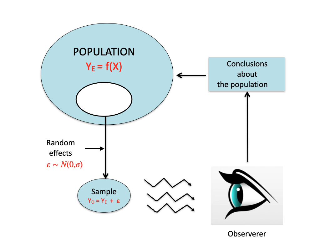
Figure 5.1: The process of experimental research: inferring the characteristics of a population by looking at a sample

In this chapter we will offer an overview about statistical inference, by using two real-life examples; the first one deals with a quantitative variable, while the second one deals with a proportion.

5.1 Example 1: a concentration value

Let’s consider again the situation we have examined in Chapter 4: a well is polluted by herbicide residues and we want to know the concentration of those residues. We plan a Monte Carlo experiment where we collect three water samples and make chromatographic analyses.

As this is a Monte Carlo experiment, we can imagine that we know the real truth: the unknown concentration is 120 mg/L and the analytic instrument is characterised by a coefficient of variability of 10%, corresponding to a standard deviation of 12 mg/L. Consequently, our observations (\(Y_i\), with \(i\) going from 1 to 3 replicates) will not match the real unknown concentration value, but they will be a random realisation, from the following Gaussian distribution (see Chapter 4):

\[Y_i \sim \textrm{Norm}(120, 12)\],

Accordingly, we can simulate the results of our experiment:

set.seed(1234)
Ye <- 120
Y <- rnorm(3, Ye, 12)
Y
## [1] 105.5152 123.3292 133.0133

Now, let’s put ourselves in the usual conditions: we have seen the results and we know nothing about the real truth. What can we learn from the data, about the concentration in the whole well?

First of all, we postulate a possible model, such as the usual model of the mean:

\[Y_i \sim \textrm{Norm}(\mu, \sigma)\]

This is the same model we used to simulate the experiment, but, in the real world, we do not know the values of \(\mu\) and \(\sigma\) and we need to estimate them from the observed data. We know that \(\mu\) and \(\sigma\) are, respectively, the mean and the standard deviation of the whole population and, therefore, we calculate these two descriptive stats for our sample and name them, respectively, \(m\) and \(s\).

m <- mean(Y)
s <- sd(Y)
m; s
## [1] 120.6192
## [1] 13.9479

Now the question is: having seen \(m\) and \(s\), can we infere the values of \(\mu\) and \(\sigma\)? Assuming that the sample is representative (we should not question this, as long as the experiment is valid), our best guess is that \(\mu = m\) and \(\sigma = s\). This process by which we assign the observed sample values to the population values is known as point estimation.

Although point estimation is totally legitimate, we clearly see that it leads to wrong conclusions: due to sampling errors, \(m\) is not exactly equal to \(\mu\) and \(s\) is not exactly equal to \(\sigma\)! Therefore, a more prudential attitude is recommended: instead of expressing our best guess as a single value, we would be much better off if we could use some sort of uncertainty interval. We need a heuristic to build such an interval.

5.1.1 The empirical sampling distribution

In this book we will use the popular heuristic proposed by Jarzy Neyman, although we need to clearly state that this is not the only one and it is not free from some conceptual inconsistencies (See Morey et al., 2016). Such a heuristic is based on trying to guess what should happen if we repeat the experiment for a very high number of times. Shall we obtain similar results or different? Instead of guessing, we exploit Monte Carlo simulation to make true repeats. Therefore:

we repeat the sampling process 100,000 times (i.e., we collect three water samples for 100,000 times and analyse their concentrations)
we get 100,000 average concentration values
we describe this population of means.

In R, we can use the code below. Please, note the iterative procedure, based on the for() statement, by which all instructions between curly brackets are repeated, while the counter \(i\) is updated at each cycle, from 1 to 100,000.

# Monte Carlo simulation
set.seed(1234)
result <- rep(0, 100000)
for (i in 1:100000){
  sample <- rnorm(3, 120, 12)
  result[i] <- mean(sample)
}
mean(result)
## [1] 120.0341
sd(result)
## [1] 6.939063

Now, we have a population of sample means and we see that:

the mean of this population is equal to the mean of the original population. It is, therefore, confirmed that the only way to obtain a perfect estimate of the population mean \(\mu\) is to repeat the experiment an infinite number of times;
the standard deviation of the population of means is equal to 6.94 and it is called standard error (SE); this value is smaller than \(\sigma\).

In order to more thouroughly describe the variability of sample means, we can bin the concentration values into a series of intervals (from 80 to 160 mg/L with a 2.5 step) and calculate the proportion of means in each interval. In this way, we build an empirical distribution of probabilities for the sample means (Figure 5.2), which is called sampling distribution. Indeed, this term has a more general importance and it is used to name the distribution of probabilities for every possible sample statistics.

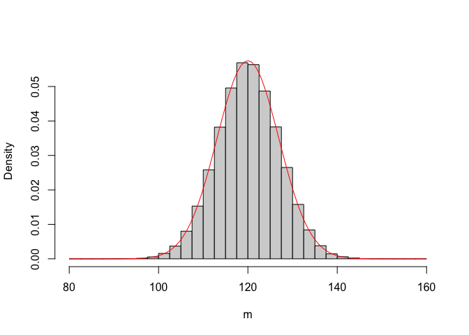
Empirical distribution of 100,000 sample means (n = 3) from a Gaussian population with mean = 120 and SD = 12. The solid line shows a Gaussian PDF, with mean = 120 and SD = 6.94

Figure 5.2: Empirical distribution of 100,000 sample means (n = 3) from a Gaussian population with mean = 120 and SD = 12. The solid line shows a Gaussian PDF, with mean = 120 and SD = 6.94

The sampling distribution and its standard error are two very important objects in research, as they are used to describe the precision of estimates: when the standard error is big, the sampling distribution is flat and our estimates are tend to be rather uncertain and highly variable across repeated experiments. Otherwise, when the standard error is small, our estimates are very reliable and precise.

5.1.2 A theoretical sampling distribution

Building an empirical sampling distribution by Monte Carlo simulation is always possible, but it may often be impractical. Looking at Figure 5.2, we see that our sampling distribution looks very much like a Gaussian PDF with mean equal to 120 and standard deviation close to 6.94.

Indeed, such an empirical observation has a theoretical support: the central limit theorem states that the sampling distribution of whatever statistic obtained from random and independent samples is approximately gaussian, whatever it is the PDF of the original population where we sampled from ¹. The same theorem proves that, if the population mean is \(\mu\), the mean of the sampling distribution is \(\mu\).

The standard deviation of the sampling distribution, in this case, can be derived by the law of propagation of errors, based on three main rules:

the sum of gaussian variables is also gaussian. Besides, the product of a gaussian variable for a constant value is also gaussian.
For independent gaussian variables, the mean of the sum is equal to the sum of the means and the variance of the sum is equal to the sum of the variances.
If we take a gaussian variable with mean equal to \(\mu\) and variance equal to \(\sigma^2\) and multiply all individuals by a constant value \(k\), the mean of the product is equal to \(k \times \mu\), while the variance is \(k^2 \times \sigma^2\).

In our experiment, we have three individuals coming from a gaussian distribution and each individual inherits the variance of the population from which it was sampled, which is \(\sigma^2 = 12^2 = 144\). When we calculate the mean, we sum the three values as the first step and the variance of the sum is \(144 + 144 + 144 = 3 \times 144 = 432\). As the second step, we divide by three and the variance of this ratio (see #3 above) is 432 divided by \(3^2\), i.e. \(432/9 = 48\). The standard error is, therefore, \(\sqrt{48} = 6.928\); it is not exactly equal to the empirical value of 9.94, but this is only due to the fact that we did not make an infinite number of repeated sampling.

In general, the standard error of a mean (SEM) is:

\[\sigma_m = \frac{\sigma}{\sqrt n}\]

Now, we can make our first conclusion: if we repeat an experiment a very high number of times, the variability of results across replicates can be described by a sampling distribution, that is (approximately) gaussian, with mean equal to the true result of our experiment and standard deviation equal to the standard error.

5.1.3 The frequentist confidence interval

If the sampling distribution is gaussian, we could take a value \(k\), so that the following expression holds:

\[P \left[ \mu - k \times \frac{\sigma}{\sqrt{n} } \leq m \leq \mu + k \times \frac{\sigma}{\sqrt{n} } \right] = 0.95\]

It means that we can build an interval around \(\mu\) that contains 95% of the sample means (\(m\)) from repeated experiments (Figure 5.3).

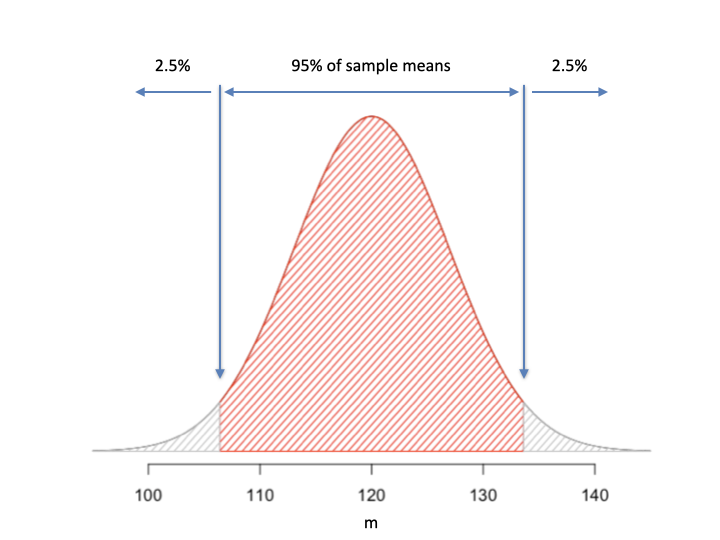
Building a confidence interval (P = 0.95): if we sample from a population with a mean of 120, 95 of our sample means out of 100 will be in the above interval

Figure 5.3: Building a confidence interval (P = 0.95): if we sample from a population with a mean of 120, 95 of our sample means out of 100 will be in the above interval

With simple math, we get to the following expression, that is of extreme importance:

\[P \left[ m - k \times \frac{\sigma}{\sqrt{n} } \leq \mu \leq m + k \times \frac{\sigma}{\sqrt{n} } \right] = 0.95\]

It says that, when we make an experiment and get an estimate \(m\), by an appropriate selection of \(k\), we can build an interval around \(m\) that is equal to \(k\) times the standard error, and contains the population value \(\mu\) with 95% probability. Here is the heuristic we were looking for!

For our example:

we calculate the sample mean. We conclude that \(\mu = m = 120.6192\) mg/L and this is our point estimate;
we calculate the standard error as \(\sigma/\sqrt{n}\). As we do not know \(\sigma\), we plug-in our best guess, that is \(s = 13.95\), so that \(SE = 13.95 / \sqrt{3} = 8.053\);
we express our uncertainty about the population mean by replacing the point estimate with an interval, given by \(\mu = 120.6192 \pm k \times 8.053\). This process is known as interval estimation.

The interval \(\mu = 120.6192 \pm k \times 8.053\) is called confidence interval and it is supposed to give us a better confidence that we are not reporting a wrong mean for the population (be careful to this: we are in doubt about the population, not about the sample!).

But, how do we select a value for the multiplier \(k\)? Let’s go by trial and error. We set \(k = 1\) and repeat our Monte Carlo simulations, as we did before. At this time, we calculate 100,000 confidence intervals and count the number of cases where we hit the population mean. The code is shown below and it is very similar to the code we previously used to build our sampling distribution.

# Monte Carlo simulation - 2
set.seed(1234)
result <- rep(0, 100000)
for (i in 1:100000){
  sample <- rnorm(3, 120, 12)
  m <- mean(sample)
  se <- sd(sample)/sqrt(3)
  limInf <- m - se
  limSup <- m + se
  if(limInf < 120 & limSup > 120) result[i] <- 1
}
sum(result)/100000
## [1] 0.57749

Indeed, we hit the real population mean only in less than 60 cases out of 100, which is very far away from 95%; we’d better widen our interval. If we use twice the standard error (\(k = 2\)), the probability becomes slightly higher than 81% (try to run the code below).

# Monte Carlo simulation - 3
set.seed(1234)
result <- rep(0, 100000)
for (i in 1:100000){
  sample <- rnorm(3, 120, 12)
  m <- mean(sample)
  se <- sd(sample)/sqrt(3)
  limInf <- m - 2 * se
  limSup <- m + 2 * se
  if(limInf < 120 & limSup > 120) result[i] <- 1
}
sum(result)/100000
## [1] 0.81708

Using twice the standard error could be a good approximation when we have a high number of degrees of freedom. For example, running the code below shows that, with 20 replicates, a confidence interval obtained as \(m \pm 2 \times s/\sqrt{3}\) hits the population mean in more than 94% of the cases. Therefore, such a confidence interval (‘naive’ confidence interval) is simple and it is a good approximation to the 95% confidence interval when the number of observations is sufficiently high.

# Monte Carlo simulation - 4
set.seed(1234)
result <- rep(0, 100000)
for (i in 1:100000){
  n <- 20
  sample <- rnorm(n, 120, 12)
  m <- mean(sample)
  se <- sd(sample)/sqrt(n)
  limInf <- m - 2 * se
  limSup <- m + 2 * se
  if(limInf < 120 & limSup > 120) result[i] <- 1
}
sum(result)/100000
## [1] 0.94099

For our small sample case, we can get an exact 95% coverage by using the 97.5-th percentile of a Student’s t distribution, that is calculated by using the qt() function in R:

qt(0.975, 2)
## [1] 4.302653

The first argument is the desired percentile, while the second argument represents the number of degrees of freedom for the standard deviation of the sample, that is \(n - 1\). The value of 4.303 can be used as the multiplier for the standard error, leading to the following confidence limits:

m + qt(0.025, 2) * s/sqrt(3)
## [1] 85.33977
m + qt(0.975, 2) * s/sqrt(3)
## [1] 154.6368

A further Monte Carlo simulation (see below) shows that this is a good heuristic, as it gives us a confidence interval with a real 95% coverage.

# Monte Carlo simulation - 4
set.seed(1234)
result <- rep(0, 100000)
for (i in 1:100000){
  sample <- rnorm(3, 120, 12)
  m <- mean(sample)
  se <- sd(sample)/sqrt(3)
  limInf <- m - qt(0.975, 2) * se
  limSup <- m + qt(0.975, 2) * se
  if(limInf < 120 & limSup > 120) result[i] <- 1
}
sum(result)/100000
## [1] 0.94936

Obviously, we can also build a 99% or whatever else confidence interval, we only have to select the right percentile from a Student’s t distribution. In general, if \(\alpha\) is the confidence level (e.g. 0.95 or 0.99), the percentile is \(1 - (1 - \alpha)/2\) (e.g., \(1 - (1 - 0.95)/2 = 0.975\) or \(1 - (1 - 0.99)/2 = 0.995\)).

5.2 Example 2: a proportion

For the previous example, we have sampled from a gaussian population, but this is not always true. Let’s imagine we have a population of seeds, which are 77.5% germinable and 22.5% dormant. If we take a sample of 40 seeds and measure their germinability, we should not necessarily obtain 31 (40 \(\times\) 0.775) germinated seeds, due to random sample-to-sample fluctuations.

Analogously to the previous example, we could think that the number of germinated seeds might show random variability, according to a gaussian PDF with \(\mu\) = 31 and a certain standard deviation \(\sigma\). However, such an assumption is not reasonable: the count of germinated seeds is a discrete variable going from 0 to 40, while the gaussian PDF is continuous from \(-\infty\) to \(\infty\). A survey of literature shows that the random variability in the number of germinated seeds can be described by using a binomial PDF (Snedecor and Cochran, 1989); accordingly, we can simulate our germination experiment by using a binomial random number generator, that is the rbinom(s, n, p) function. The first argument represents the number of experiments we intend to request, the second represents the number of seeds under investigation in each experiment, while the third one represents the proportion of successes in the population (we can take the germination as a success). Let’s simulate the results of an experiment:

set.seed(1234)
nGerm <- rbinom(1, 40, 0.775)
nGerm
## [1] 34
nGerm/40
## [1] 0.85

We see that we get 34 germinated seeds, corresponding to a proportion \(p = 34/40 = 0.85\). Looking at the observed data, what can we conclude about the proportion of germinable seeds for the whole population? Our point estimate, as usual, is \(\pi = p = 0.85\), but we see that this is expectedly wrong; how could we calculate a confidence interval around this point estimate? Can we use the same heuristic as we did before for concentration data?

Let’s use Monte Carlo simulation to explore the empirical sampling distribution. We repeat the experiment 100,000 times and we obtain 100,000 proportions with which we build an empirical sampling distribution (see the code below, showing the sampled proportions for the first six experiment). How does the sampling distribution look like?

res <- rbinom(100000, 40, 0.775)/40
head(res)
## [1] 0.750 0.750 0.750 0.700 0.750 0.925
mean(res)
## [1] 0.7749262
sd(res)
## [1] 0.06611151

Unsurprisingly, Monte Carlo simulation leads us to an approximately normal sampling distribution for \(p\), as implied by the central limit theorem (Figure 5.4). Furthermore, the mean of the sampling distribution is 0.775 and the standard deviation is 0.066.

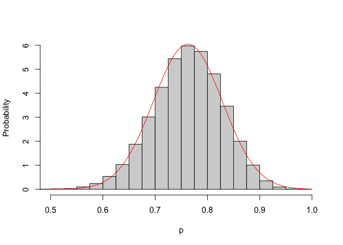
Figure 5.4: Monte Carlo sampling distribution for the proportion of germinable seeds, when the population proportion is 0.775

We can conclude that the confidence interval for an estimated proportion can be calculated in the very same way as for the mean, with the only difference that the standard error is obtained as \(\sigma_p = \sqrt{p \times (1 - p)}/\sqrt(n)\) (Snedecor and Cochran, 1989). Consequently, using the observed data, \(p = 0.85\) and \(s = \sqrt{0.85 \times 0.15} = 0.357\); our confidence interval is \(0.85 \pm 2 \times 0.357/sqrt(40)\) and we can see that, by reporting such an interval, we have correctly hit our population proportion. In this case the size of our sample was big enough (40) to use \(k = 2\) as the multiplier.

5.3 Conclusions

The examples we used are rather simple, but they should help to understand the process:

we have a population, from which we sampled the observed data;
we used the observed data to calculate a statistic (mean or proportion);
we inferred that the population statistic was equal to the sample statistic (e.g., \(\mu = m\) or \(\pi = p\));
we estimated a standard error for our sample statistic, by using either Monte Carlo simulation, or by using some simple function, depending on the selected statistic (e.g. \(\sigma/\sqrt{n}\) for the mean and \(\sqrt{p \times (1 - p)}/\sqrt(n)\) for the proportion);
we used a multiple of the standard error to build a confidence interval around our point estimate.

We will use the same process throughout this book, although the sample statistics and related standard errors will become slightly more complex, as we progress towards the end. Please, do not forget that the standard error and confidence interval are fundamental components of science and should always be reported along with every point estimate.

Last, but not least, it is important to put our attention on the meaning of the so-called ‘frequentist’ confidence interval:

it is a measure of precision
it relates to the sampling distribution; i.e. we say that, if we repeat the experiment a high number of times and, at any times, we calculate the confidence interval as shown above, we ‘capture’ the real unknown parameter value in 95% of the cases
it does not refer to a single sampling effort

Points 2 and 3 above imply that confidence intervals protect ourselves from the risk of reaching wrong conclusions only in the long run. In other words, the idea is that, if we use such a heuristic, we will not make too many mistakes in our research life, but that does not imply that we are 95% correct in each experimental effort. Indeed, a single confidence interval may contain or not the true population mean, but we have no hint to understand whether we hit it or not. Therefore, please, remember that such expressions as: “there is 95% probability that the true population parameter is within the confidence interval” are just abused and they should never find their way in any scientific manuscripts or reports.

5.4 Further readings

Hastie, T., Tibshirani, R., Friedman, J., 2009. The elements of statistical learning, Springer Series in Statistics. Springer Science + Business Media, California, USA.
Morey, RD, R Hoekstra, JN Rouder, MD Lee, E-J Wagenmakers, 2016. The fallacy of placing confidence in confidence intervals. Psychonomic Bulletin & Review 23, 103–123
Snedecor G.W. and Cochran W.G., 1989. Statistical Methods. Ames: Iowa State University Press (1989).

The central limit theorem holds for very large samples. With small samples, the approximation is good only with more than 15-20 units↩︎