Chapter 2 Designing experiments
The interest I have in believing a thing is not a proof of the existence of that thing (Voltaire)
2.1 The elements of research
In the previous chapter we have seen that every valid experiment should adhere to three fundamental principles, i.e. control, replication and randomisation. You may wonder: how do we put such principles into practice? Of course, there is not an easy and general answer: setting up a good experiment is mainly a matter of experience and the tuition of an experienced colleague is essential, especially while moving the first steps in the research world.
In this chapter, we will focus on some common elements that we need to care about for all experiments, of any type. These elements are:
- the hypothesis and objectives;
- the experimental treatments;
- the experimental units;
- the allocation of treatments to units;
- the response variables.
All detail about those elements need to be clearly given at the beginning of every good research project, report or scientific manuscript.
2.2 Hypothesis and objectives
The Galilean process of research starts from a well founded hypothesis, i.e. a predictive statement about the possible outcome of a certain biological system. Such an hypothesis is usually based on an accurate review of literature information and, possibly, on a set of preliminary experiments. It must be:
- relevant;
- clearly defined;
- specific;
- testable.
A well set hypothesis leads naturally to the definition of the objectives of the experiment, which must be:
- realistic;
- achievable;
- measurable;
- time constrained.
Objectives should always be phrased in such a way that it is possible to exactly identify the moment when they have been achieved. For complex research projects, involving more than one experiment, it may be useful to define a general objective and several specific objectives, organised in successive phases, so that it is easy to check the progress of the research study and to revise the time schedule, in case some unexpected problems arise.
Unclear objectives may lead to inefficient research, wherein unnecessary data are collected, while relevant observations are left out.
2.3 The experimental treatments
Once the objectives are clear, we need to define the experimental ‘stimuli’ that will be allocated to the experimental units. A set of related ‘stimuli’ is called the experimental factor; for example, if we want to compare the genotypes A, B and C, we have the genotype factor with three levels. If we have one factor with a unique level, we usually talk about mensurative experiment, otherwise, we talk about comparative experiment, which is, by far, the most common situation.
2.3.1 Factorial experiments
When we have two (or more) experimental factors, we could either make separate experiments, or we could make a factorial experiment, wherein we combine the levels of the two factors. This second solution is much more interesting, because we can assess possible interaction effects between the two factors (we will talk about this in Chapter 12).
Factorial experiments may be planned in two different ways, i.e. they can be crossed or nested. In a crossed design, we have all possible combinations between the levels for all factors; for example, if we want to compare three sunflower genotypes (A, B and C) at two different nitrogen rates (N1 and N2), a crossed factorial experiment should include all the six combinations A-N1, A-N2, B-N1, B-N2, C-N1 and B-N2. Otherwise, in a nested design, the levels of one factor are different, depending on the level of the other factor; for example, if we want to compare organic farming and conventional farming by using the most suitable maize genotypes for each agricultural system, we should use a nested design.
Recognising crossed and nested factorial designs is important, because the resulting data needs to be analysed in different ways.
2.3.2 The control
Very often, comparative experiments need a suitable control or check level, which is used as the reference against which all other treatments are evaluated. We can include either:
- an untreated control,
- a control treated with a placebo, or
- a control treated with ordinary practices.
For example, in a genotype experiment we usually include a reference genotype that is very widely grown in all nearby farms. For herbicide experiments, we always include an untreated control, which is fundamental to assess the composition of weed flora and quantify weed control efficacy for all herbicides under investigation. Furthermore, we can also include a weed-free control (usually hand-weeded) as the reference to evaluate possible symptoms of herbicide phytotoxicity to the crop. In toxicology, the untreated control may be replaced by a control treated with a placebo, i.e. a compound containing the same components of the experimental treatment, except the active ingredient. The placebo is usually necessary when:
- the experimental subject (usually a human) perceives its condition and reacts to the expectation about the efficacy of the chemical under investigation;
- the commercial formulation, apart from the active ingredient, contains other components, such as adjuvants, surfactants and other substances which may show some sort of biological effects.
2.4 The experimental units
The experimental unit is the physical entity to which the treatment is allocated, e.g. a plant, a plot, an animal, a pot. In this respect, we need to be careful to clearly distinguish the experimental units from the observational units; indeed, we can allocate the treatment to a field plot and measure several plants therein or we can allocate the treatment to a tree and measure several leaves on that tree. A clear distinction between experimental units and observational units can help us avoid problems with pseudo-replication (see Chapter 1).
The experimental units are always selected from a wider population of interest. For example, we select the plots from a field, the plants from a crop or some animals from a herd. A sample should be representative and homogeneous, although these may be two contrasting characteristics. Indeed, if we select very homogeneous individuals, we run the risk of getting a sample that no longer represents the whole population, but only a subset of it. For example, if our sample was composed by adult male bovines in good health, it may not necessarily represent a population composed also by females, young and diseased animals. Sampling a population of interest in a proper way may be a daunting task, especially in the social sciences. Several sampling protocols have been defined (e.g., random sampling, systematic sampling, stratified sampling, clustered sampling, convenience sampling, quota sampling, …), which are far beyond the scope of this book; you can read Daniel (2011) for a thorough explanation.
In some cases, the process of sampling is less obvious, but that does not mean that there is no sampling. For example, in manipulative laboratory experiments, the experimental units are specifically prepared for each assay, such as the pots for a herbicide assay or the Petri dishes for a germination assay. Even if there is no real selection process, these units should be regarded as sampled from the wider population of pots or Petri dishes that we could have possibly prepared.
2.5 The allocation of treatments
Unless we select experimental units that are ‘naturally treated’ (observational experiments; see Chapter 1), one central issue of every experiment is the technique we use to allocate the treatments. In general, following Fisher’s principles, we should pursue a completely randomised allocation, although, in some circumstances, it may be advantageous to put some constraints, as long as such constraints are not neglected during the process of data analysis. Constraints are very common in field experiments and we will see that they set the basis for the so-called experimental layout.
In some cases, it is appropriate to hide some detail of the allocation process; for example, in medical research, it may be necessary that the subjects are not aware about which treatment they are going to receive (single-blind experiments), in order to avoid possible unconscious effects. In agriculture, it is often necessary that the researcher is not aware about which treatment was allocated to each unit, in order to avoid that the objectivity of visual and sensory assessments is undermined. If neither the subjects nor the researcher are aware about the treatment, we talk about double-blind experiments.
2.6 The variables
At the end of an experiment we produce a set of data (dataset), which is composed by a collection of variables. These variables describe the experimental units in relation to some of their characteristics and we usually distinguish (i) response variables, (ii) factor variables and (iii) accessory variables.
The response variables, obviously, describe the response of units to the experimental treatments (e.g., the yield, the weight, the height, and so on), while the factor variables describe the experimental stimulus allocated to each unit (e.g., the tillage method, fertilisation rate, genotype and so on). In some cases, we also record other accessory variables (or covariates), which measure potential confounding effects. For example, if we intend to study the yield of a number of trees, depending on how they are fertilised, the effect of tree age can act as a confounder. Therefore, if we cannot use trees of the same age, we can record the age as an accessory variable and use it to obtain a more reliable assessment of the fertilisation effect.
It is useful to classify the variables depending on their characteristics, into
- nominal variables;
- ordinal variables;
- count/ratio variables;
- continuous variables.
2.6.1 Nominal variables
Nominal variables are produced by assigning the subjects to a set of categories, such as dead/alive, germinated/ungerminated, red/blue/green, and so on. The categories can be two (binomial response) or more (multinomial response), they should not have any intrinsic ordering and should be mutually exclusive, in the sense that one individual can only belong to one category. With these variables, we can only count the number of individuals in each category (frequency), while other descriptive stats such as the mean and standard deviation are not used, at least not in the usual sense.
2.6.2 Ordinal variables
Ordinal variables are similar to nominal variables, but the categories are intrinsically ordered. For example, we could ask a farmer to express his appreciation for a certain agronomic practice, by using five categories, VERY LOW, LOW, AVERAGE, HIGH and VERY HIGH. The categories are mutually exclusive and ordered by increasing appreciation; thanks to such an ordering, we can calculate both the frequency in each category and the cumulative frequency, which is obtained by summing the frequency in each category to the frequencies in all the preceding categories (see next Chapter). With ordinal variables, descriptive statistics such as the mean can, sometimes, be calculated, as long as the distance between the categories is clearly defined.
2.6.3 Count and ratio variables
Sometimes the experimental units are characterised by some countable property; therefore, we can obtain a count for each unit and, consequently, a count variable. Please, note that this is different from a nominal/ordinal variable, where we count the units, not a specific trait in each single unit. For example, we obtain a count variable when we count the number of weeds in a plot, or the number of germinated seeds in a Petri dish, or the number of fruits per plant. When those counts have a predefined plateau, we can express them as relative to the plateau and obtain a ratio variable. For example, if we have ten seeds in a Petri dish, the count of germinated seeds may not exceed ten and it can be expressed as the proportion of germinated seeds. Both count and ratio data are discrete, in the sense that they can only take certain values (they are not continuous), but the mean and other descriptive stats can be be easily calculated with the usual method (see next Chapter).
2.6.4 Continuous variables
Continuous variables can take any value within a certain interval, such as the weight, height, yield, time and so on. It could be argued that every measurement instrument is characterised by its own resolution, below which all measurements take the same value. Therefore we could say that all continuous variable are, in practice, discrete. However, we can neglect this detail, as long as the resolution is high enough for practical purposes.
Continuous variables give a lot of information, although, in some instances, we may be interested in transforming them into ordinal variables, by using a classification procedure: we subdivide the range in classes (e.g. < 50, 50-100, 100-150, > 150) and count the number of individuals in each class. This is often useful for descriptive purposes with big data, as we will see in the following chapter.
2.6.5 Sensory and visual assessments
In some instances, instead of measuring a certain trait of interest, we make visual or sensory assessments. For example, weed control ability and selectivity of herbicides can be assessed either by counting or weighing the survived weeds or by visual observations on a scale from 0 to 100% (or similar scales). Sensory and visual assessments are rather common and give several advantages, such as:
- low cost,
- high speed,
- no need for costly instruments,
- the possibility of disregarding the effect of external confounders. For example, when scoring the effect of an herbicide, an expert technician can easily distinguish phytotoxic effects from water stress damage and, thus, he can only consider the former effects, which would be impossible with objective weight measurements.
Of course, there are also several disadvantages, such as:
- lower precision
- subjectivity
- we can be unconsciously influenced by knowing how the experimental unit has been treated
- it may be difficult to keep a uniform judgment parameter throughout the survey
- we need experience and training
Sensory and visual data are largely acceptable in science, although their analysis may require some extra care and specific methods. Indeed, the resulting variable may resemble an ordinal variable (we assign one of a set of ordered categories), although the underlying scale is more or less continuous.
2.7 Setting up a field experiment
Once all the elements of an experiment have been carefully planned, we must be laid down such an experiment in practice. The techniques greatly vary depending on the disciplines, aims, scales (climatic chamber, greenhouse, laboratory, field and so on) and it is very difficult to provide general information, apart from reinforcing the idea that all valid experiments must controlled, replicated and randomised, as detailed in the previous chapter.
In this part, we will focus on the peculiar traits of field experiments, although most of the information relating to the experimental lay-out also applies to other types of experiments.
2.7.1 Selecting the field
Field selection is perhaps the key aspect for a successful experiment. First of all, a research field must be close enough to roads, laboratories and other facilities, which will permit a timely execution of sampling and measurements.
Secondly, we should not forget that there are countless reasons why a field experiment may turn out inconclusive, due to very wide environmental variability, relating to soil, weather, pests and so on. Therefore, at the onset of every experiment, we need to ensure that those sources of variability are kept to a minimum level, by selecting a very homogeneous field. We need to stay away from field parts with water stagnation, ditches, rows of trees and any other elements inducing an increase of variability in the behaviour of field crops.
Knowing the history of the field may also be rather important. Some previous crops (e.g., alfalfa or other legumes) may leave excess fertility in soil, which is not good if, e.g., a N-fertilisation experiment is to be set-up. Likewise, herbicide trials may leave non-homogeneous infestation levels, due to the presence of untreated controls and other low efficacy herbicides. The history of a field is also important, for herbicide and pest management experiments, as we may be interested in having/avoiding a certain weed or pest in our field.
If we suspect that there might be problems with soil heterogeneity, we should take some appropriate preliminary actions, such as growing a oat catch crop to remove excess soil nitrogen, growing alfalfa or other forage crops to suppress weed growth or perform deep ploughing to reduce the weed seed bank in the uppermost soil layer.
In order to enhance crop homogeneity, small plot experiments (see later) should be managed by suitable machinery, that is optimised to work on small surfaces; furthermore, some interventions (such as sowing, weeding and fertilising) can also be performed by hand. A peculiar technique that is often used to obtain a homogeneous crop density is sowing at overly high density and thin out to optimal density a few days after crop emergence.
2.7.2 Selecting the units within the field
Once we have selected a suitable field, we need to identify the experimental units. In this respect, we should distinguish:
- demonstrative on-farm trials
- small plot research trials
Demonstrative trials usually represent the final stage of research and they are usually conducted on commercial farms under realistic environmental and management conditions, considering all the inherent variability of farming systems. The aim is usually to obtain a reliable validation of new products, managements and technologies at the farm level; therefore, the experimental unit is usually the strip, i.e. a long, rectangular piece of land, wherein the usual farming machinery (plough, planters, sprayers, combine harvester and so on) can be used.
The number of treatments under comparison is low and, most often, one new management practice (e.g. crop management, crop protection, plant nutrition, and plant growth regulator) is compared to a local/farmer ‘control’ in two contiguous strips. Such pair (the new management practice and the control) is a replicate; normally we should have a minimum of three (more is better) replicates for capturing within-field variability. For the sake of simplicity, considering the size of strips, randomisation may be omitted, so that the design resembles the type A-3 in Figure 1.4 (see previous chapter). One possible lay-out is shown in Figure 2.1, where we have four fields with two strips each; in one field, the first strip is assigned to one treatment and the second strip is assigned to the other.
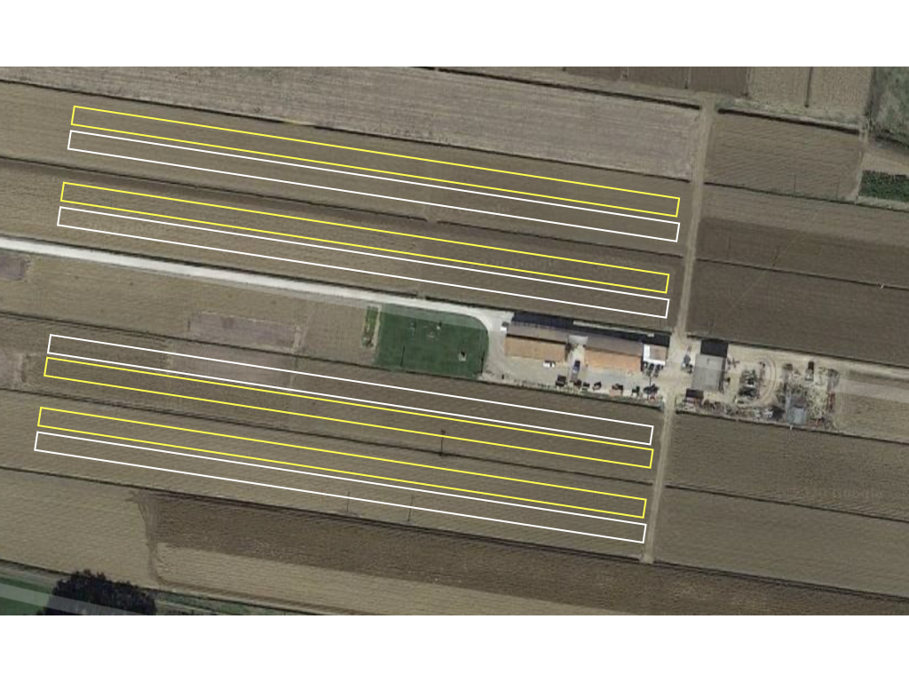
Figure 2.1: The possible lay out of an on-farm trial, with four fields, two strips per field and a different treatment per strip (yellow and white)
On-farm experiments are repeated across locations and growing seasons, so that we can have a better confidence in the selection of improved agronomic practices in new environments.
On the other hand, small plot experiments are in the middle between on-farm and laboratory experiments: they are set up in the field, but the experimental unit is represented by a plot, i.e. a small piece of land, usually of 10 to 50 m\(^2\) surface (Figure 2.2). In small plot experiments we can keep a high degree of control for most confounding factors, while working in close-to-real conditions, which explains why this type of experiments is very widespread in the agricultural sciences. Of course, the observed yields in small plot experiments are usually 10-30% higher than the corresponding yields in on-farm conditions, due to more careful management of all cropping practices.
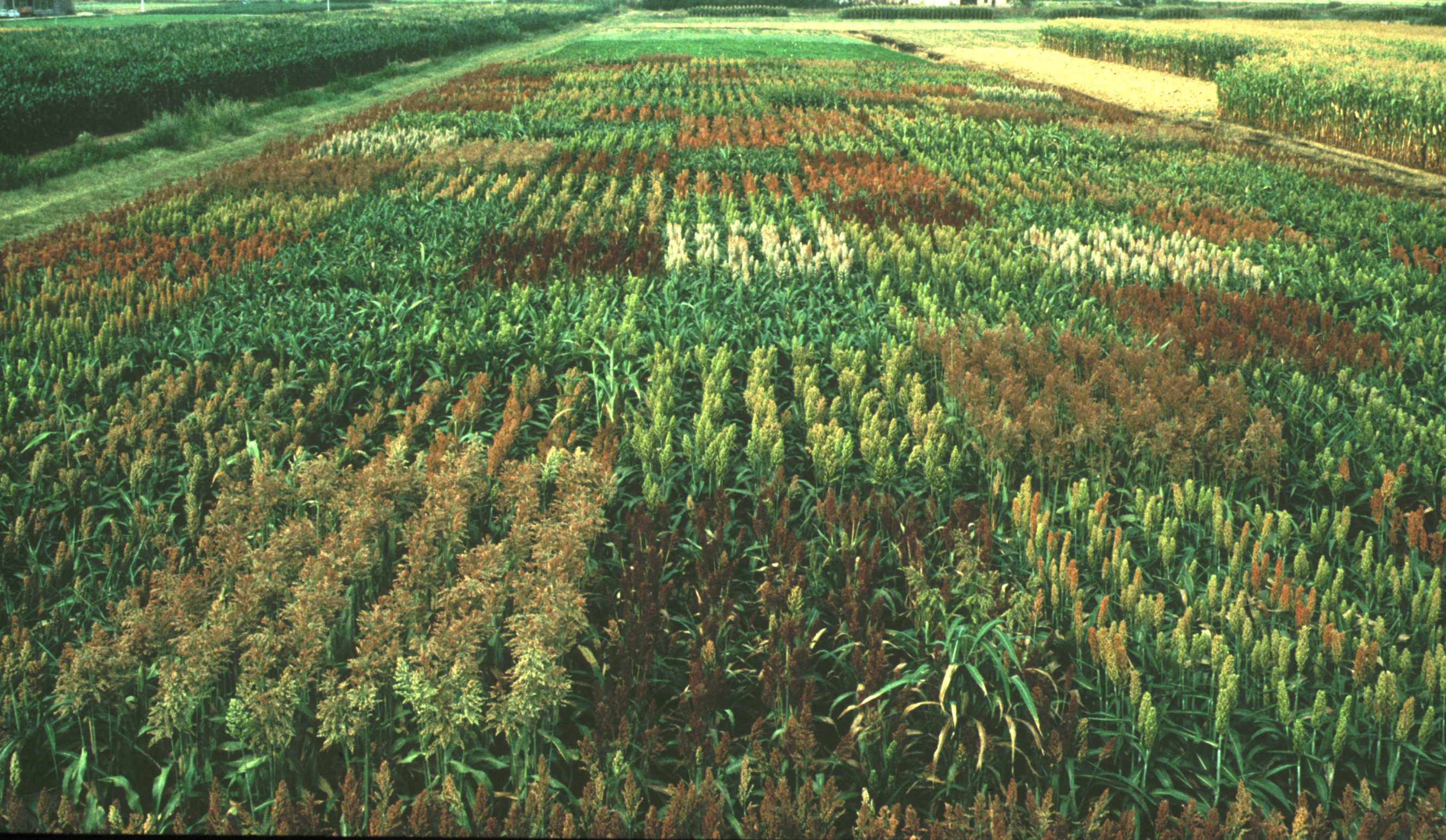
Figure 2.2: A small plot experiment in the field (Ph. D. Alberati)
Considering the shape, we usually prefer rectangular plots, where the width is equal to a multiple of the width of the available machinery for sowing and harvesting. Plot size must be big enough to accommodate a sufficiently high number of plants; for low density crops (e.g. maize), 20-40 m2 minimum are usually required, while for high density crops (e.g. wheat or alfalfa) 10-20 m2 may suffice. Smaller plots may not produce representative results, but, unless we are planning on-farm experiments, bigger plots can also be disadvantageous, as the plot-to-plot variability is increased. If we have a big field at our disposal, we might prefer to increase the number of replicates, instead of increasing the size of plots.
When selecting plot shape and size we should consider the presence of border effects, that represent an important source of variability. Indeed, plant growing along the plot edges are not in the same conditions as plants in the middle of each plot; for example, they might be more vigorous and productive, because of the lack of competition on one side. Or, they might be affected by, e.g., the carry-over effects of fertilisers and herbicides across neighbouring plots. Border effects need to be minimised by restricting all measurements to the central rows of each plot, while the plants along the edges are omitted. This way, the surface area for harvest is smaller than the total plot surface area, which should be taken into account while designing the experiment.
2.7.3 Number of replicates
For field experiments, the number of replicates is usually set to 3 to 5. A lower number of replicates is not to be recommended, because the experiment becomes very inefficient. On the other hand, a higher number of replicates increases the time and cost requirements and may result in increased soil variability and decreased precision. Once we have selected the number of replicates, the total number of plots is obtained as the product of the number of treatment levels and the number of replicates.
2.7.4 The field map
The layout of a field experiment is usually planned in a map (field map), showing the lay-out of plots within the field. An example is shown in Figure 2.3, relating to an experiment with eight treatments and four replicates (32 plots, in total). In order to maximise the homogeneity, we have laid down the plots in eight vertical strips with four plots each. The plots are characterised by a rectangular shape and they are 8 m long and 2 m wide, which makes up a surface area of 16 m2. Around the experiment, we added 24 additional plots, in order to minimise border effects along the edges of the experiment. An arrow pointing towards the North is included, so that we can appropriately orient our map, during the field inspections. All plots are clearly identified by a univocal numbering/coding system.
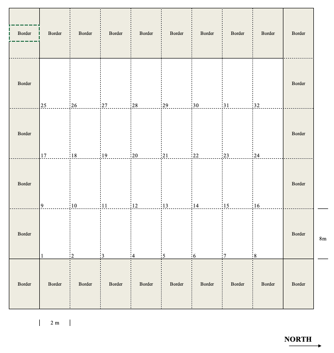
Figure 2.3: Example of a field map for an experiment with 32 plots
2.7.5 The experimental lay-out
We can use the map to project the allocation of treatments to the units. While the basic principle of randomisation needs to always be followed, the experimental lay-out can be different, according to our organisational needs. The following lay-outs are very common in agriculture, although we will show that they can be used also in experiments of other types.
2.7.5.1 Completely randomised design (CR)
With this design, treatments are allocated to plots in a completely randomised fashion, in strict accordance with Fisher’s rule. An example is shown in Figure 2.4, where we have allocated 8 treatments (the letters from A to H) with four replicates to the 32 plots in Figure 2.3.
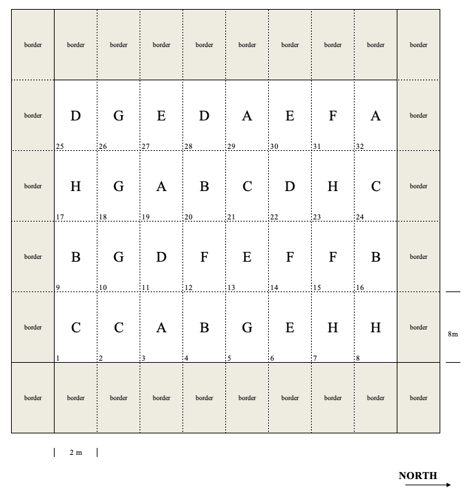
Figure 2.4: Example of an experiment laid down as a completely randomised design
Such an approach is very simple and always correct, although it has the disadvantage that every possible systematic source of heterogeneity goes unnoticed. For example, let’s imagine that, for some reasons, the first three plot columns in Figure 2.4 (plots 1, 2, 3, 9, 10, 11, 17, 18, 19, 25, 26 and 27) are more fertile than all the other columns. In this case, the treatment G is favoured, because three out of four replicates are located in the most fertile part, while the treatment H is penalised, because only one replicate is in that most fertile part.
Therefore, CRDs are very common in laboratory/greenhouse experiments or in field experiments characterised by a high degree of environmental, soil and crop homogeneity.
2.7.5.2 Randomised complete block design (RCBD)
In RCBDs, the experimental units are divided into homogeneous groups with as many subjects as there are treatments to be allocated. The division is made according to some innate characteristic of subjects, such as age, sex, proximity; for field experiments, we usually exploit some expected fertility gradients. For example, should we expect a left-to-right fertility gradient for the plots in Figure 2.3, we could divide the experiment in four blocks with two plot columns each (8 plot per each block; block 1 would, e.g., contain the plots 1, 9, 17, 25, 2, 10, 18 e 26). Subsequently, we could randomly allocate the eight treatments to the plots in each block, so that there is one replicate per block. By doing so, no treatment should be penalised/favoured (Figure 2.5)
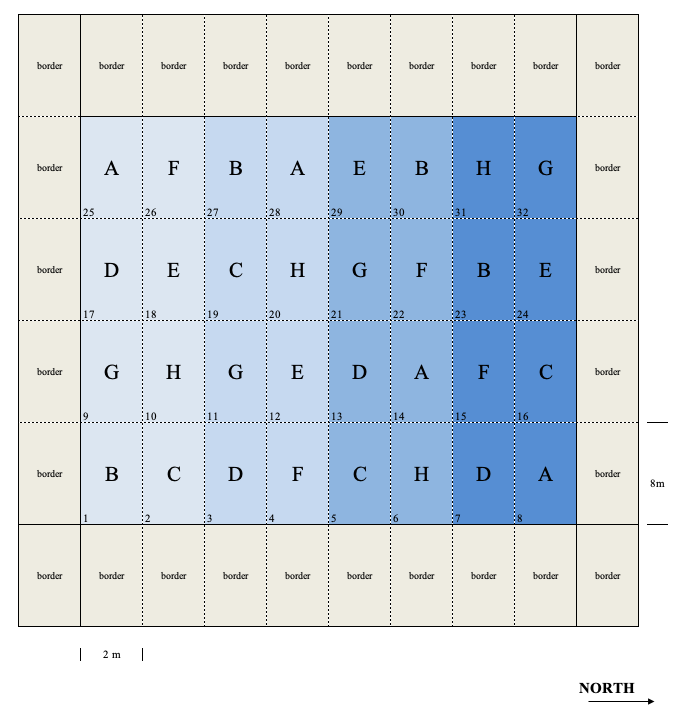
Figure 2.5: Example of a completely randomised block design
RCBD is the most common design for field experiments, although it can be used wherever the experimental units can be divided in groups, according to some innate property. In the following chapters we will see that the RCBD is very efficient when the variability across blocks is very big, as a big part of the subject-to-subject variability can be accounted for and removed from the unexplained variation.
2.7.5.3 Latin square design
In some cases, the experimental units can be grouped according to two innate properties, apart from the experimental treatments. Figure 2.6 shows a design with 4 treatments and four replicates (16 plots in all); if we assume that there are a left-to-right and a bottom-to-top fertility gradients, we can look at the rows and columns as different blocking variables. Therefore, we can allocate the treatments to plots, so that there is one replicate in each row and in each column.
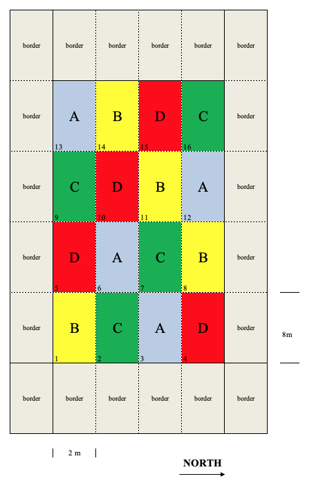
Figure 2.6: Example of a latin square design with four treatments (A, B, C and D) and four replicates. The different colours help identify the four treatments and their allocation to the plots.
Latin square designs are not only useful for field experiments. For example, if we want to test the effect of four different working protocols in the time required to accomplish a certain task, we can use a number of workers as the experimental units. In order to have four replicates, we need 16 workers, to which we allocate the different protocols, according to a CRD or CRBD. We can reduce the number of workers by allowing each worker to use all four protocols, in four subsequent shifts. For example, the first worker can use the protocols A, B, C and D, one after the other in a randomised order. By doing so, we only need four workers and the experiment is designed as CRBD, where the worker acts as a blocking factor. The advantage is that possible worker-to-worker differences in proficiency are not confounded with differences between protocols, as all workers use all protocols.
However, we should also consider that workers tend to get tired over time and loose proficiency and, therefore, the protocols used at the beginning of the sequence are favoured with respect to the protocols used later on. We can account for this effect by allocating the protocols in a way that each one is used in all shifts; as the consequence, the shift acts as the second blocking factor, as shown in Figure 2.7. This is, indeed, a latin square design.
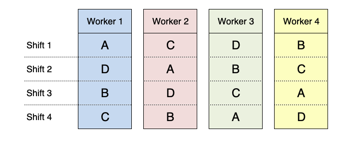
Figure 2.7: Example of a latin square design for the comparison of four working protocols, by using four workers and four turns.
The latin square takes its name from the fact that the number of replicates is equal to the number of treatments and, therefore, the field map consists of a square grid, where each treatment can be found in all rows and all columns (some of you may recognise the basic principle of the Sudoku game…). It is a useful design, as it can account for possible plot-to-plot differences in relation to two blocking factors (rows and columns, or workers and turns), so that the unexplained plot-to-plot differences are minimised. The disadvantage is that the number of replicates must be equal to the number of treatments and, therefore, the latin square can only be used for experiments with few treatments.
2.7.5.4 Split-plot and strip-plot designs
With factorial experiments we can simply use a CRD or RCBD, by allocating the combinations of all factor levels to the different plots. For example, think about an experiment to compare three types of tillage (minimum tillage = MIN; shallow ploughing = SP; deep ploughing = DP) and two types of chemical weed control methods (broadcast = TOT; in-furrow = PART). With four replicates, the six treatment combinations (MIN-TOT, SP-TOT, DP-TOT, MIN-PART, SP-PART and DP-PART) can be allocated to 24 plots, according to a RCBD, as shown in Figure 2.8. Please note that we had to allow a wide space between the plots, in order to permit the circulation of tractors and tillage machinery.
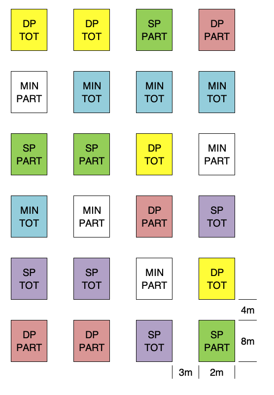
Figure 2.8: Field map for a two-factor factorial experiment, laid down as RCBD
For those who have some knowledge with field research, it may be obvious that tillage treatments require big plots and a wide space between plots, due to the size of tillage machinery. On the contrary, spraying herbicides may be easily done also on small plots. Therefore, we could think of using big plots to allocate tillage treatments and splitting these big plots into two subplots, to allocate weed control treatments (split-plot design). The example is shown in Figure 2.9: we note that the allocation of tillage treatments to the 12 main-plots is done according to a RCBD, while the two weed control treatments are randomly allocated to the two sub-plots, within each main-plot.
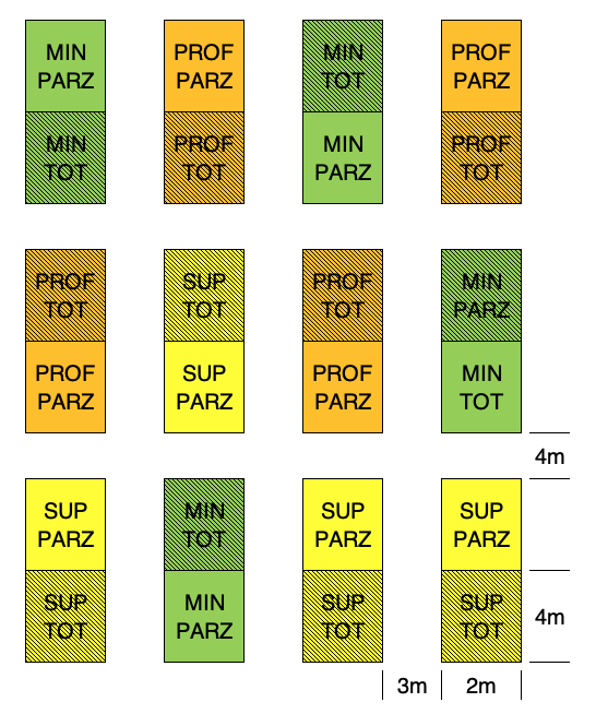
Figure 2.9: Same design as in the previous Figure, laid down as split-plot.
An important consequence of split-plot designs is that every main-plot represents a replicate for sub-plot factor levels; indeed, if we look at Figure 2.9, we see that there are four replicates for each tillage level, but there are 12 replicated sub-plots for each weed control level. Therefore, subplot effects are estimated with higher precision.
As all other designs, split-plot designs are not specific to agriculture experiments and they find their place in many other research topics. In general, they are used whenever:
- one factor require bigger experimental units, as in the above shown example;
- the levels for one factor are difficult to allocate and it is preferable to manipulate groups of experimental units, instead of a single independent experimental unit. For example, we might be interested in studying the corrosion resistance of steel bars treated with four coatings at three furnace temperatures. This latter factor is hard to change, as it takes a long time to reach a new equilibrium temperature within the furnace. Therefore, once the equilibrium temperature is reached, it is convenient to put four steel bars with each of the four coatings inside the furnace and record their corrosion. We repeat the process at the three temperatures and repeat the whole experiment twice. This is an example of a split-plot experiment, where temperatures are allocated to a furnace (main-plot) and coatings are allocated the steel bars (sub-plots).
A useful variant of the split plot is used when the treatments are allocated in strips (strip-plot designs), as shown in Figure 2.10. This map refers to an experiment where three crops were sown 40 days after a herbicide treatment, in order to assess possible phytotoxicity effects relating to an excessive persistence of herbicide residues. We see that each block is organised with three rows and two columns: the three crops were sown along the rows and the two herbicide treatments (rimsulfuron and the untreated control) were allocated along the columns. The combinations are, consequently, allocated to subplots. In this design, we have three types of plots: the row-plots, the column-plots and the subplots; the advantage is that the allocation of treatments is rather quick.
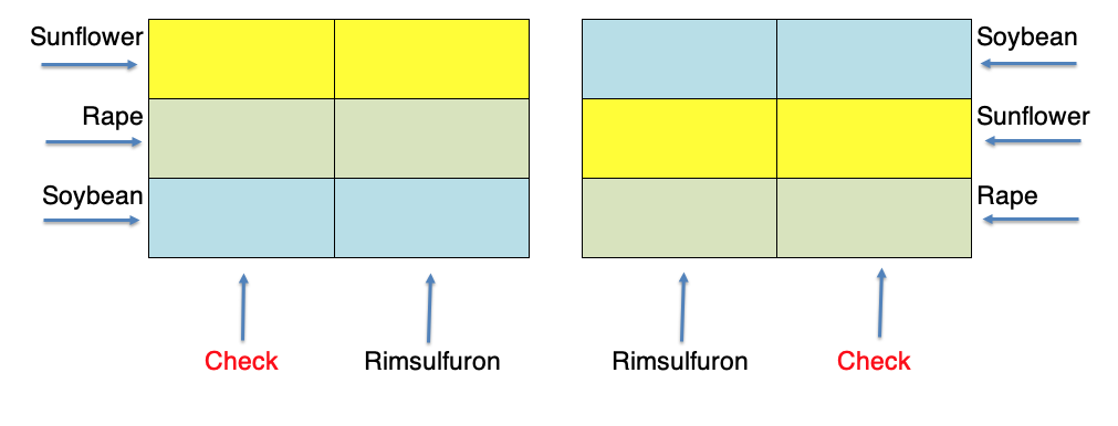
Figure 2.10: Same design as in the previous Figure, laid down as strip-plot.
2.8 Conclusions
In this chapter we have seen the fundamental elements of a research and we have also seen how those elements, considering the three fundamental characteristics of control, replication and randomisation, can be joined together to set-up valid experiments in the field. We have also seen that the different types of designs are commonly used also for laboratory experiments or other types of experiments outside agriculture.
2.9 Further readings
- Cochran, W.G., Cox, G.M., 1950. Experimental design. John Wiley & Sons, Inc., Books.
- Daniel, J. 2011. Sampling Essentials: Practical Guidelines for Making Sampling Choices. USA: SAGE.
- LeClerg, E.L., Leonard, W.H., Clark, A.G., 1962. Field Plot Technique. Burgess Publishing Company, Books.
- Jones, B., Nachtsheim, C.J., 2009. Split plot designs: what, why and how. Journal of Quality Technology 41, 340–361.