Chapter 8 Checking for the basic assumptions
An approximate answer to the right problem is worth a good deal more than an exact answer to an approximate problem (J. Tukey)
Let’s take a further look at the ANOVA model we fitted in the previous chapter:
\[Y_i = \mu + \alpha_j + \varepsilon_i\]
with:
\[ \varepsilon_i \sim N(0, \sigma) \]
The above equations imply that the random components \(\varepsilon_i\) (residuals) are the differences between observed and predicted data:
\[\varepsilon_i = Y_i - Y_{Ei}\]
where:
\[Y_{Ei} = \mu + \alpha_j\]
By definition, the mean of residuals is always 0, while the standard deviation \(\sigma\) is to be estimated.
As all the other linear models, ANOVA models make a number of important assumptions, which we have already listed in the previous chapter. We repeat them here:
- the deterministic model is linear and additive (\(\mu + \alpha_j\));
- there are no other effects apart from the treatment and random noise. In particular, there are no components of systematic error;
- residuals are independently sampled from a gaussian distribution;
- the variance of residuals is homogeneous and independent from the experimental treatments (homoscedasticity assumption)
The independence of residuals and the absence of systematic sources of experimental errors are ensured by the adoption of a valid experimental design and, therefore, they do not need to be checked after the analyses. On the contrary, we need to check that the residuals are gaussian and homoscedastic: if the residuals do not conform to such assumptions, the sampling distribution for the F-ratio is no longer the Fisher-Snedecor distribution and our P-values are invalid.
In this respect, we should be particularly concerned about strong deviations, as the F-test is rather robust and can tolerate slight deviations with no dramatic changes of P-values.
8.1 Outlying observations
In some instances, deviations from the basic assumptions can be related to the presence of outliers, i.e. ‘odd’ observations, very far away from all other observations in the sample. For example, if the residuals are gaussian with mean equal to zero and standard deviation equal to 5, finding a residual of -20 or lower should be rather unlikely (32 cases in one million observations), as shown by the pnorm() function in the box below:
The presence of such an unlikely residual in a lot of, e.g., 50 residuals should be considered as highly suspicious: either we were rather unlucky, or there is something wrong with that residual. This is not irrelevant: indeed, such an ‘odd’ observation may have a great impact on the estimation of model parameters (means and variances) and hypothesis testing. This would be a so-called influential observation and we should not let it go unnoticed. We suggest that, before checking for the basic assumptions, a careful search for the presence of outliers should never be forgotten.
8.2 The inspection of residuals
The residuals of linear models can be inspected either by graphical methods, or by formal hypothesis testing. Graphical methods are simple, but they are powerful enough to reveal strong deviations from the basic assumptions (as we said, slight deviations are usually tolerated). We suggest that these graphical inspection methods are routinely used with all linear models, while the support of formal hypothesis testing is left to the most dubious cases.
Residuals can be plotted in various ways, but, in this section, we will present the two main plot types, which are widely accepted as valid methods to check for the basic assumptions.
8.2.1 Plot of residuals against expected values
First of all, it is useful to plot the residuals against the expected values. If there are no components of systematic error and if variances are homogeneous across treatments, the points in this graph should be randomly scattered (Figure 8.1 ), with no visible systematic patterns.
Every possible deviation from such a random pattern should be carefully inspected. For example, the presence of outliers is indicated by a few ‘isolated points’, as shown in Figure 8.2.
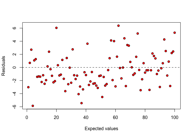
Figure 8.1: Plot of residuals against expected values: there is no visible deviation from basic assumptions for linear model
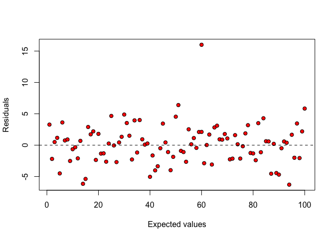
Figure 8.2: Plot of residuals against expected values: an outlying observation is clearly visible
When the cloud of points takes the form of a ‘fennel’ (Figure 8.3), the variances are proportional to the expected values and, therefore, they are not homogeneous across treatments (heteroscedasticity).
In some other cases, the residuals tend to be systematically negative/positive for small expected values and systematically positive/negative for high expected values (Figure 8.4). Such a behaviour may be due to some unknown sources of systematic error, which is not accounted for in the deterministic part of the model (lack of fit). Such a behaviour is not very common with ANOVA models and we postpone further detail until the final two book chapters.
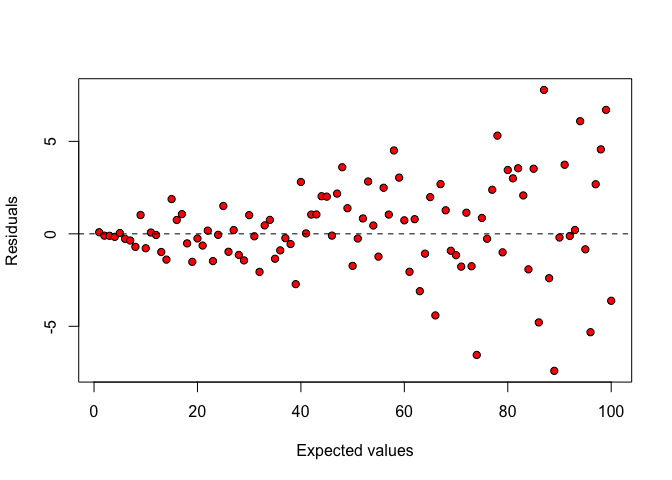
Figure 8.3: Plot of residuals against expected values: heteroscedastic data.
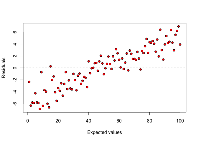
Figure 8.4: Plot of residuals against expected values: lack of fit
8.2.2 QQ-plot
Plotting the residuals against the expected values let us discover the outliers and gives us evidence of heteroscedastic errors; however, it does not suggest whether the residuals are gaussian distributed or not. Therefore, we need to draw the so-called QQ-plot (quantile-quantile plot), where the standardised residuals are plotted against the respective percentiles of a normal distribution. But, what are the respective percentiles of a gaussian distribution?
I will not go into detail about this (you can find information in my blog, at this link), but I will give you an example. Let’s imagine we have 11 standardised residuals sorted in increasing order: how do we know whether such residuals are drawn from a gaussian distribution? The simplest answer is that we should compare them with 11 values that are, for sure, drawn from a standardised gaussian distribution.
With eleven values, we know that the sixth value is the median (50th percentile), while we can associate to all other values the respective percentage point by using the ppoints() function, as shown in the box below:
pval <- ppoints(1:11)
pval
##  [1] 0.04545455 0.13636364 0.22727273 0.31818182 0.40909091 0.50000000
##  [7] 0.59090909 0.68181818 0.77272727 0.86363636 0.95454545
We see that the first observation corresponds the 4.5th percentile, the second observation is the 13.63th percentile and so on, until the final observation that is the 95.45th percentile. What are these percentiles in a standardised gaussian distribution? We can calculate them by using the qnorm() function:
perc <- qnorm(pval)
perc
##  [1] -1.6906216 -1.0968036 -0.7478586 -0.4727891 -0.2298841  0.0000000
##  [7]  0.2298841  0.4727891  0.7478586  1.0968036  1.6906216
If our 11 standardised residuals are gaussian, they should match the behaviour of the respective percentiles in a gaussian population: the central residual should be close to 0, the smallest one should be close to -1.691, the second one should be close to -1.097 and so on. Furthermore, the number of negative values should be approximately equal to the number of positive values and the median should be approximately equal to the mean.
Hence, if we plot our standardised residuals against the respective percentiles of a standardised gaussian distribution, the points should lie approximately along the diagonal, as shown in Figure 8.5, for a series of residuals which were randomly sampled from a gaussian distribution.
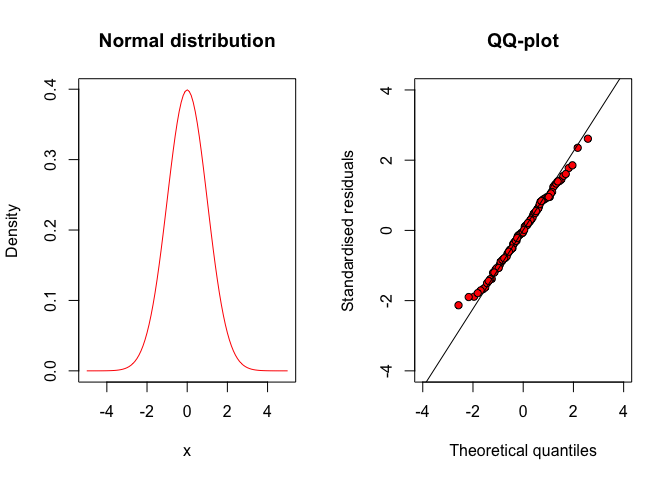
Figure 8.5: QQ-plot for a series of gaussian residuals
Any deviations from the diagonal suggests that the residuals do not come from a normal distribution, but they come from other distributions with different shapes. For example, we know that the gaussian distribution is symmetric, while residuals might come from a right-skewed distribution (leaning to the left). In such asymmetric distribution, the mean is higher than the median and negative residuals are more numerous, but lower in absolute value than positive residuals (see Figure 8.6, left). Therefore, the QQ-plot looks like the one in Figure 8.6(right).
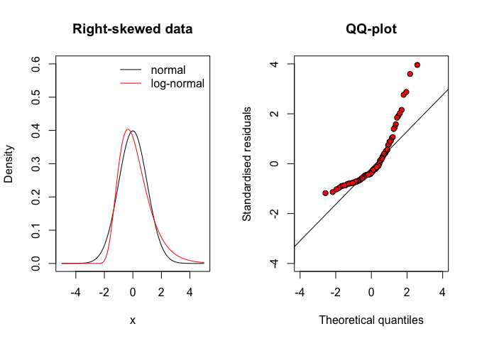
Figure 8.6: QQ-plot for residuals coming from a right-skewed distribution (e.g., shifted log-normal)
Otherwise, when the residuals come from a left-skewed distribution (asymmetric and leaning to the right), their mean is lower than the median and there are a lot of positive residuals with low absolute values (Figure 8.7, left). Therefore, the QQ-plot looks like that in Figure 8.7 (right).
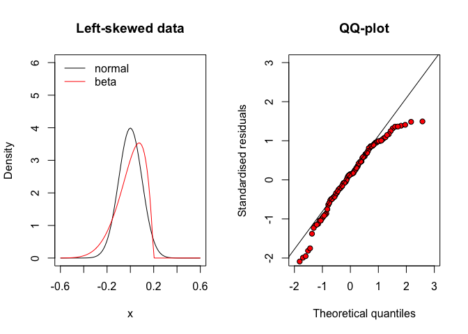
Figure 8.7: QQ-plot for residuals coming from a left-skewed distribution (e.g., a type of beta distribution)
Apart from symmetry, the deviations from a gaussian distribution may also concern the density in both the tails of the distribution. In this respect, the residuals may come from a platicurtic distribution, where the number of observations far away from the mean (outliers) is rather high, with respect to a gaussian distribution (Figure 8.8, left). Therefore, the QQ-plot looks like the one in Figure 8.8 (right). Otherwise, when the residuals come from a leptocurtic distribution, the number of observations far away from the mean is rather low (see Figure 8.9 and the QQ-plot looks like that in Figure 8.9 (right).
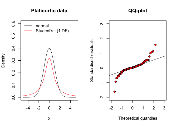
Figure 8.8: QQ-plot for residuals coming from a platicurtic distribution (e.g., the Student’s t distribution with few degrees of freedom)
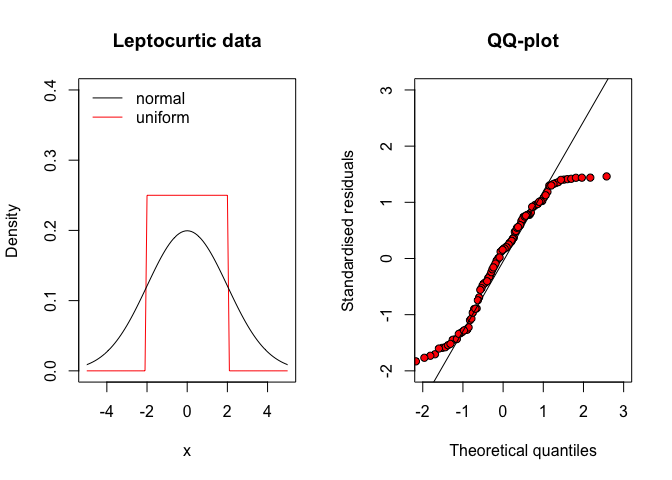
Figure 8.9: QQ-plot for residuals coming from a leptocurtic distribution (e.g., a uniform distribution)
8.3 Formal hypotesis testing
Graphical methods usually reveal the outliers and the most important deviations from basic assumptions. However, we might be interested in formally testing the hypothesis that there are no deviations from basic assumptions (null hypothesis), by using some appropriate statistic. Nowadays, a very widespread test for variance homogeneity is the Levene’s test, which consists of fitting an ANOVA model to the residuals as absolute values. The rationale is that the residuals sum up to zero within each treatment group; if we remove the signs, the residuals become positive, but the group means tend to become higher when the variances are higher. For example, we can take two samples with means equal to zero and variances respectively equal to 1 and 4.
A <- c(0.052, 0.713, 1.94, 0.326, 0.019, -2.168, 0.388,
       -0.217, 0.028, -0.801, -0.281)
B <- c(3.025, -0.82, 1.716, -0.089, -2.566, -1.394,
       0.59, -1.853, -2.069, 3.255, 0.205)
mean(A); mean(B)
## [1] -9.090909e-05
## [1] 6.308085e-17
var(A); var(B)
## [1] 1.000051
## [1] 4.000271
mean(abs(A))
## [1] 0.6302727
mean(abs(B))
## [1] 1.598364
Taking the absolute values, the mean for A is 0.63, while the mean for B is 1.60. We see that the second mean is higher than the first, which is a sign that the two variances might not be homogeneous. If we submit to ANOVA the absolute values, the difference between groups is significant, which leads to the rejection of the homoscedasticity assumption. In R, the Levene’s test can also be performed by using the leveneTest() function in the ‘car’ package.
res <- c(A, B)
treat <- rep(c("A", "B"), each = 11)
model <- lm(abs(res) ~ factor(treat))
anova(model)
## Analysis of Variance Table
##
## Response: abs(res)
##               Df  Sum Sq Mean Sq F value Pr(>F)
## factor(treat)  1  5.1546  5.1546  5.8805 0.0249 *
## Residuals     20 17.5311  0.8766
## ---
## Signif. codes:  0 '***' 0.001 '**' 0.01 '*' 0.05 '.' 0.1 ' ' 1
car::leveneTest(res ~ factor(treat), center = mean)
## Levene's Test for Homogeneity of Variance (center = mean)
##       Df F value Pr(>F)
## group  1  5.8803 0.0249 *
##       20
## ---
## Signif. codes:  0 '***' 0.001 '**' 0.01 '*' 0.05 '.' 0.1 ' ' 1
The Levene’s test can also be performed by considering the medians of groups instead of the means (‘center = median’), which gives us a more robust test, i.e. less sensible to possible outliers.
Possible deviances with respect to the gaussian assumption can be tested by using the Shapiro-Wilks’ test. For example, taking 100 residuals from a uniform distribution (i.e. a non-gaussian distribution) and submitting them to the Shapiro-Wilks’ test, the null hypothesis is rejected with P = 0.0004.
8.4 What do we do, in practice?
Now, it’s time to take a decision: do our data meet the basic assumptions for ANOVA? A wide experience in the field suggests that a decision is hard to take in most situations. Based on experience, our recommendations are:
- a thorough check of the residuals should never be neglected;
- be very strict when the data come as counts or ratios: for this type of data the basic assumptions are very rarely met and, therefore, you should consider them as non-normal and heteroscedastic whenever you have even a small sign to support this;
- be very strict with quantitative data, when the differences between group means are very high (higher than one order of magnitude); for this data, variances are usually proportional to means and heteroscedasticity is the norm and not the exception;
- for all other data, you can be slightly more liberal, without neglecting visible deviations from basic assumptions.
8.5 Correcting measures
Whenever our checks suggest important deviations from basic assumptions, we are supposed to take correcting measures, otherwise our analyses are invalid. Of course, correcting measures change according to the problem we have found in our data.
8.5.1 Removing outliers
If we have found an outlier, the simplest correcting strategy is to remove it. However, we should refrain from this behaviour as much as possible, especially when sample size is small. Before removing an outlier we should be reasonably sure that it came as the consequence of some random error or intrusion, without being, anyhow, related to the effect of some treatments.
For example, if we are making a genotype experiment and one of the genotypes is not resistant to a certain fungi disease, in the presence of such disease we might expect that yield variability for the sensible genotypes increases and, therefore, the presence of occasional plots with very low yield levels becomes more likely. In this case, outliers are not independent on the treatment and removing them is wrong, because relevant information is hidden.
In all cases, please, remember that removing data points to produce a statistically significant result is regarded as a terribly bad practice! Furthermore, by definition, outliers should be rare: if the number of outliers is rather high, we should really think about discarding the whole experiment and making a new one.
8.5.2 Stabilising transformations
After having considered and managed the presence possible outliers, the most traditional method to deal with data that do not conform to the basic assumptions for linear models is to transform the response into a metric that is more amenable to linear model fitting. In particular, the logarithmic transformation is often used for counts and proportions, the square root transformation is also used for counts and the arcsin-square root transformation is very common with proportions.
Instead of making an arbitrary selection, we suggest the procedure proposed by Box and Cox (1964), that is based on the following family of transformations:
\[ W = \left\{ \begin{array}{ll} \frac{Y^\lambda -1}{\lambda} & \quad \textrm{if} \,\,\, \lambda \neq 0 \\ \log(Y) & \quad \textrm{if} \,\,\, \lambda = 0 \end{array} \right.\]
where \(W\) is the transformed variable, \(Y\) is the original variable and \(\lambda\) is the transformation parameter. We may note that, apart from a linear shift (subtracting 1 and dividing by \(\lambda\), which does not change the distribution of data), if \(\lambda = 1\) we do not transform at all. If \(\lambda = 0.5\) we make a square-root transformation, while if \(\lambda = 0\)2 we make a logarithmic transformation; furthermore, if \(\lambda = -1\) we transform into the reciprocal value.
Box and Cox (1964) gave a method to calculate the likelihood of the data under a specific \(\lambda\) value, so that we can try several \(\lambda\) values and see which one corresponds to the maximum likelihood value. Accordingly, we can select this maximum likelihood \(\lambda\) value and use it for our transformation. We’ll give an example of such an approach later on.
8.7 Example 1
First of all, let’s check the dataset we have used in the previous chapter (‘mixture.csv’). We load the file and re-fit the ANOVA model, by using the ‘Weight’ as the response and the herbicide treatment ‘Treat’ as the treatment factor.
repo <- "https://www.casaonofri.it/_datasets/"
file <- "mixture.csv"
pathData <- paste(repo, file, sep = "")

dataset <- read.csv(pathData, header = T)
head(dataset)
##             Treat Weight
## 1 Metribuzin__348  15.20
## 2 Metribuzin__348   4.38
## 3 Metribuzin__348  10.32
## 4 Metribuzin__348   6.80
## 5     Mixture_378   6.14
## 6     Mixture_378   1.95
dataset$Treat <- factor(dataset$Treat)
mod <- lm(Weight ~ Treat, data = dataset)
After fitting, we can get the graphical analyses of residuals by using the plot() method on the model object; the argument ‘which’ can be set to 1 or 2: the former value produces a plot of residuals against expected values, while the latter value produces a QQ-plot of residuals. The syntax is as follows:
plot(mod, which = 1)
plot(mod, which = 2)
The output is shown in Figure 8.10.
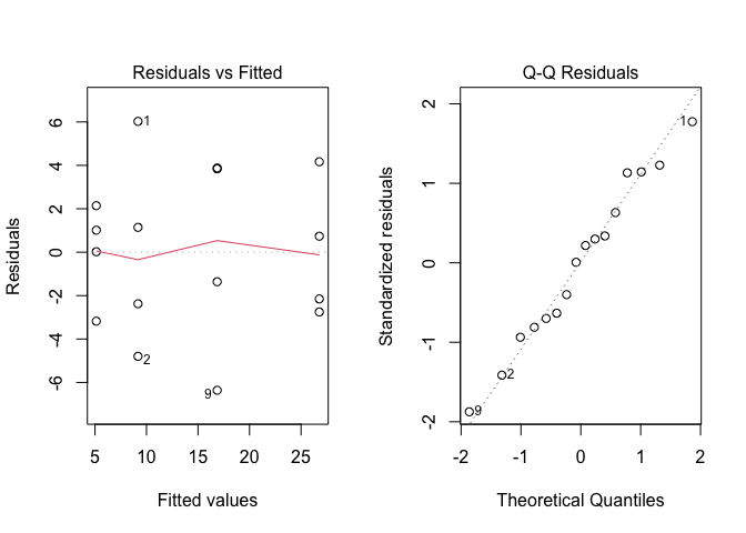
Figure 8.10: Graphical analyses of residuals for the ‘mixture.csv’ dataset
None of the two graphs suggests deviations from the basic assumptions. Considering that we have a quantitative variable with small differences (less than one order of magnitude) between group means, we skip all formal analyses and conclude that we have no reasons to fear about the basic assumptions for linear models.
8.8 Example 2
Let’s consider the dataset in the ‘insects.csv’ file. Fifteen plants were treated with three different insecticides (five plants per insecticide) according to a completely randomised design. A few weeks after the treatment, we counted the eggs of insects over the leaf surface. In the box below we load the dataset and fit an ANOVA model, considering the variables ‘Count’ as the response and ‘Insecticide’ as the experimental factor.
file <- "insects.csv"
pathData <- paste(repo, file, sep = "")
dataset <- read.csv(pathData, header = T)
head(dataset)
##   Insecticide Rep Count
## 1          T1   1   448
## 2          T1   2   906
## 3          T1   3   484
## 4          T1   4   477
## 5          T1   5   634
## 6          T2   1   211
mod <- lm(Count ~ Insecticide, data = dataset)
Now we plot the residuals, by using the ‘plot’ method, as shown above, The output is reported in Figure 8.11.
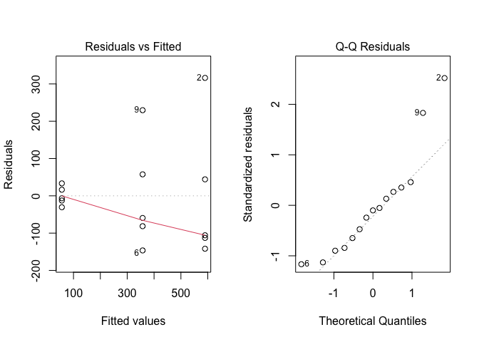
Figure 8.11: Graphical analyses of residuals for the ‘insects.csv’ dataset
In this case we see clear signs of heteroscedastic (left plot) and right-skewed residuals (right plot). Furthermore, the fact that we are working with counts encourages a more formal analysis. The Levene’s test confirms our fears and permits to reject the null hypothesis of homoscedasticity (P = 0.043). Likewise, the hypothesis of normality is rejected (P = 0.048), by using a Shapiro-Wilks test. The adoption of some correcting measures is, therefore, in order.
car::leveneTest(mod, center = mean )
## Warning in leveneTest.default(y = y, group = group, ...): group
## coerced to factor.
## Levene's Test for Homogeneity of Variance (center = mean)
##       Df F value  Pr(>F)
## group  2   3.941 0.04834 *
##       12
## ---
## Signif. codes:  0 '***' 0.001 '**' 0.01 '*' 0.05 '.' 0.1 ' ' 1
shapiro.test(residuals(mod))
##
##  Shapiro-Wilk normality test
##
## data:  residuals(mod)
## W = 0.87689, p-value = 0.04265
We decide to use a stabilising transformation and run the boxcox() function to select the maximum likelihood value for \(\lambda\); the syntax below results in the output shown in Figure 8.12.
library(MASS)
boxcox(mod)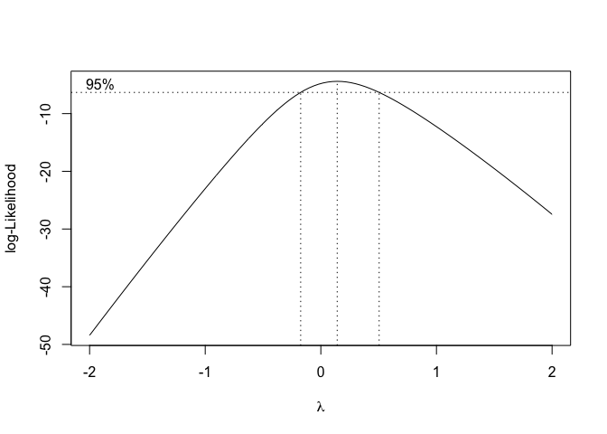
Figure 8.12: Selecting the maximum likelihood value for the transformation parameter lambda, according to Box and Cox (1964)
The graph shows that the maximum likelihood value is \(\lambda = 0.14\), although the confidence limits go from slightly below zero to roughly 0.5. In conclusion, every \(\lambda\) value within the interval \(-0.1 < \lambda < 0.5\) can be used for the transformation. We select \(\lambda = 0\), that corresponds to a logarithmic transformation, which is very widely known and understood.
In practice, we transform the data into their logarithms, re-fit the model and re-analyse the new residuals.
modt <- lm(log(Count) ~ Insecticide, data = dataset)
par(mfrow = c(1,2))
plot(modt, which = 1)
plot(modt, which = 2)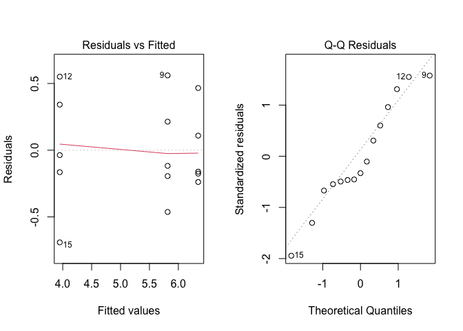
Figure 8.13: Graphical analyses of residuals for the ‘insects.csv’ dataset, following logarithmic transformation of the response variable
The situation has sensibly improved and, therefore, we go ahead with the analyses and request the ANOVA table.
anova(modt)
## Analysis of Variance Table
##
## Response: log(Count)
##             Df  Sum Sq Mean Sq F value    Pr(>F)
## Insecticide  2 15.8200  7.9100  50.122 1.493e-06 ***
## Residuals   12  1.8938  0.1578
## ---
## Signif. codes:  0 '***' 0.001 '**' 0.01 '*' 0.05 '.' 0.1 ' ' 1
The above table suggests that there are significant differences among insecticides (P = 1.493e-06). It may be interesting to compare the above output with the output obtained from the analysis of untransformed data:
anova(mod)
## Analysis of Variance Table
##
## Response: Count
##             Df Sum Sq Mean Sq F value    Pr(>F)
## Insecticide  2 714654  357327  18.161 0.0002345 ***
## Residuals   12 236105   19675
## ---
## Signif. codes:  0 '***' 0.001 '**' 0.01 '*' 0.05 '.' 0.1 ' ' 1
Apart from the fact that this latter analysis is wrong, because the basic assumptions of linear models are not respected, we can see that the analysis on transformed data is more powerful, in the sense that it results in a lower P-value. In this example, the null hypothesis is rejected both with transformed and with untransformed data, but in other situations, whenever the P-value is close to the borderline of significance, making a wise selection of the transformation becomes fundamental.
8.9 Other possible approaches
Stabilising transformations were very much in fashion until the ’80s of the previous century. At that time, computing power was limiting and widening the field of application for ANOVA models used to be compulsory. Nowadays, R and other software permit the use of alternative methods of data analysis, that allow for non-gaussian errors. These methods belong to the classes of Generalised Linear Models (GLM) and Generalised Linear Least squares models (GLS), which are two very flexible classes of models to deal with non-normal and heteroscedastic residuals.
In other cases, when we have no hints to understand what type of frequency distribution our residuals are sampled from, we can use nonparametric methods, which make little or no assumptions about the distribution of residuals.
GLM, GLS and non-parametric methods are pretty advanced and they are not considered in this introductory book.
8.10 Further readings
- Ahrens, W. H., D. J. Cox, and G. Budwar. 1990, Use of the arcsin and square root trasformation for subjectively determined percentage data. Weed science 452-458.
- Anscombe, F. J. and J. W. Tukey. 1963, The examination and analysis of residuals. Technometrics 5: 141-160.
- Box, G. E. P. and D. R. Cox. 1964, An analysis of transformations. Journal of the Royal Statistical Society, B-26, 211-243, discussion 244-252.
- D’Elia, A. 2001, Un metodo grafico per la trasformazione di Box-Cox: aspetti esplorativi ed inferenziali. STATISTICA LXI: 630-648.
- Saskia, R. M. 1992, The Box-Cox transformation technique: a review. Statistician 41: 169-178.
- Weisberg, S., 2005. Applied linear regression, 3rd ed. John Wiley & Sons Inc. (per il metodo ‘delta’)
Note that the limit of \((Y^\lambda -1)/\lambda\) for \(\lambda \rightarrow 0\) is \(\log(y)\)↩︎