Chapter 13 A brief intro to mixed models

… the actual and physical conduct of an experiment must govern the statistical procedure of its interpretation (R. A. Fisher)

Although the previous chapters have covered the analysis of data from a wide array of agricultural experiments, there are still a few important situations, which require some more advanced knowledge. In particular, we have, so far, encountered only the so-called fixed factors. An experimental factor is ‘fixed’ when its levels are purposely selected (not sampled), repeatable (we could make a new experiment with the very same levels) and of unique and direct interest, in the sense that we are not interested in any other level apart from those we have decided to include in the experiment. As we have seen in the previous chapters, fixed factors produce fixed effects, which can be expressed as differences (increases/decreases) with respect to the overall mean. Models containing only fixed effects and the residual random error term are named fixed models.

Apart from fixed factors, experiments in agriculture and biology may require the inclusion of random factors, that produce effects of random nature. An experimental factor is ‘random’ when its levels are not interesting in themselves, but they are sampled from a wider population of possible levels. Even if the levels are selected on purpose, they are, anyway, not ‘repeatable’ in the sense that, if we repeat the experiment, we cannot select the very same factor levels.

As an example of a random factor, we can imagine that we are interested in studying the variability of yield in a certain environment and, to this aim, we sample twenty representative fields at random within that environment to measure the yield level. The field factor is random, in the sense that we are not specifically interested in those twenty fields, but we are interested in the overall variability that the field effect produces on yield. Provided that the levels of the yield factor are not interesting in themselves, estimating their fixed effects (increase/decrease with respect to the overall mean) is meaningless; on the contrary, we are more interested in estimating the amount of variability, as measured by the corresponding variance (variance component). Models containing random factors together with fixed factors and the residual error term are named mixed models and, since the advent of personal computers in the 70s of the previous century, they represent a very important class of models, which require specific algorithms and fitting methods.

Mixed models are far beyond the scope of this book; for those who are interested in this subject, we recommend the wonderful book ‘Linear mixed-effects models using R: a step-by-step approach’ (Gałecki and Burzykowski, 2013). In this chapter we will only give a few examples relating to several common types of field experiments, that require the inclusion of random effects and, thus, the adoption of mixed models.

13.1 Split-plot or strip-plot experiments

We have seen in Chapter 2 that factorial experiments can be designed as split-plots or strip-plots, where treatment levels are allocated to the experimental units in groups. We have seen that this is advantageous in some circumstances, e.g., when one of the factors is better allocated to bigger plots, compared to the other factor. When factor levels are allocated to groups of individuals, the independency of residuals is broken, as the individuals within the group are more alike than the individuals in different groups. For example, let’s consider a field experiment: if one group of plots is, e.g., more fertile than the other groups, all plots within that group will share such a positive effect and, therefore, their yields will be correlated. In this case, we talk about intra-class correlation, that is a similar concept to the Pearson correlation, which we have encountered in Chapter 3.

In order to respect the basic assumption of independent residuals, data from split-plot and strip-plot experiments cannot be analysed by using the methods proposed in Chapter 11 (multi-way ANOVA models), but they require a different approach.

13.1.1 Example 1: a split-plot experiment

In chapter 2, we presented an experiment to compare three types of tillage (minimum tillage = MIN; shallow ploughing = SP; deep ploughing = DP) and two types of chemical weed control methods (broadcast = TOT; in-furrow = PART). This experiment was designed in four complete blocks with three main-plots per block, split into two sub-plots per main-plot; the three types of tillage were randomly allocated to the main-plots, while the two weed control treatments were randomly allocated to sub-plots (see Figure 2.9).

The results of this experiment are reported in the ‘beet.csv’ file, that is available in the online repository. In the following box we load the file and transform the explanatory variables into factors.

dataset <- read.csv("https://www.casaonofri.it/_datasets/beet.csv", header=T)
dataset$Tillage <- factor(dataset$Tillage)
dataset$WeedControl <- factor(dataset$WeedControl)
dataset$Block <- factor(dataset$Block)
head(dataset)
##   Tillage WeedControl Block  Yield
## 1     MIN         TOT     1 11.614
## 2     MIN         TOT     2  9.283
## 3     MIN         TOT     3  7.019
## 4     MIN         TOT     4  8.015
## 5     MIN        PART     1  5.117
## 6     MIN        PART     2  4.306

By looking at the map in Figure 2.9, it is easy to see that there are two types of constraints to randomisation:

1. each replicate of the six combinations was allocated to each block
2. the two weed control methods were allocated to each main plot

As the consequence, apart from treatment factors, we have two blocking factors, i.e. the blocks and the main-plots within each block; both this blocking factors should be included in the model, in order to ensure the independence of residuals.

13.1.1.1 Model definition

Considering the above comments, a linear model for a two-way split-plot experiment is:

\[Y_{ijk} = \mu + \gamma_k + \alpha_i + \theta_{ik} + \beta_j + \alpha\beta_{ij} + \varepsilon_{ijk}\]

where \(\gamma\) is the effect of the \(k\)^th block, \(\alpha\) is the effect of the \(i\)^th tillage, \(\beta\) is the effect of \(j\)^th weed control method, \(\alpha\beta\) is the interaction between the \(i\)^th tillage method and \(j\)^th weed control method. Apart from these effects, which are totally the same as those used in Chapter 11, we also include the main-plot effect \(\theta\), where we use the \(i\) and \(k\) subscripts, as each main-plot is uniquely identified by the block to which it belongs and by the tillage method with which it was treated (see Figure 2.9). Obviously, the main plots can be labelled in any other way, as long as each one is uniquely identified.

Now, let’s concentrate on the main-plots and forget the sub-plots for awhile; we see that the split-plot design in Figure 2.9, without considering the sub-plots, is totally similar to a Randomised Complete Block Design. Consequently, we are not really interested in the main-plots we have included in the experiment, they are simply a random sample selected from a wider universe. Furthermore, the differences between main-plots treated alike (same tillage method), once the block effect has been removed, are only due to random factors, as there is no other known systematic source of variability. Last, but not least, the levels of the tillage factor were independently allocated to main-plots, which, therefore, represent true-replicates for this factor. If we consider all previous comments, we have to conclude that the main-plot factor has to be regarded as a random factor.

Likewise, the subplot effect is also random, as subplots were sampled from a wider universe and the differences between sub-plots treated alike (same ‘tillage by weed control method’ combination) are only due to random effects (unknown sources of variability). In the end, in split-plot designs we have two random factors and, consequently, two random effects: \(\theta\) (main-plot effect) and \(\varepsilon\) (sub-plot effect), which are assumed as gaussian, with means equal to 0 and standard deviations equal to, respectively, \(\sigma_{\theta}\) and \(\sigma\). Therefore, we need to fit a mixed model.

13.1.1.2 Model fitting with R

First of all, we need to build a new variable to uniquely identify the main plots. We can do this by using numeric coding, or, more easily, by creating a new factor that combines the levels of block and tillage; we have already anticipated that each main plot is uniquely identified by the block and the tillage method.

dataset$mainPlot <- with(dataset, factor(Block:Tillage))

Due to the presence of two random effects, we cannot use the lm() function for model fitting, which is only able to accomodate one residual random term. In R, there are several mixed model fitting function; in this book, we propose the use of the lmer() function, which requires two additional packages, i.e. ‘lme4’ and ‘lmerTest’. These two packages need to be installed, unless we have already done so and loaded in the environment before model fitting.

The syntax of the lmer() function is rather similar to that of the lm() function, although the random main-plot effect is entered by using the ‘1|’ operator and it is put in brackets, in order to better mark the difference with fixed effects. See the box below for the exact coding.

# install.packages("lme4")  #only at first time
# install.packages("lmerTest")  #only at first time
library(lme4)
library(lmerTest)
mod.split <- lmer(Yield ~ Block + Tillage * WeedControl +
                  (1|mainPlot), data=dataset)

As usual, the second step is based on the inspection of model residuals. The plot() method applied to the ‘lmer’ object only returns the graph of residuals against fitted values (Figure 13.1), while there is no quick way to obtain a QQ-plot. Therefore, we use the Shapiro-Wilks test for normality, as shown in Chapter 8.

shapiro.test(residuals(mod.split))
## 
##  Shapiro-Wilk normality test
## 
## data:  residuals(mod.split)
## W = 0.93838, p-value = 0.1501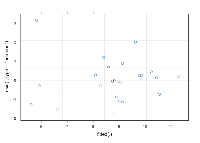

Figure 13.1: Graphical analyses of residuals for a split-plot ANOVA model

After having made sure that the basic assumptions for linear models hold, we can proceed to variance partitioning. In this case, we use the anova() method for a mixed model object, which gives a slightly different output than the anova() method for a linear model object. As the second argument, it is necessary to indicate the method we want to use to estimate the degrees of freedom, which, in mixed models, are not as easy to calculate as in linear models.

anova(mod.split, ddf="Kenward-Roger")
## Type III Analysis of Variance Table with Kenward-Roger's method
##                      Sum Sq Mean Sq NumDF DenDF F value  Pr(>F)  
## Block                3.6596  1.2199     3     6  0.6521 0.61016  
## Tillage             23.6565 11.8282     2     6  6.3228 0.03332 *
## WeedControl          3.3205  3.3205     1     9  1.7750 0.21552  
## Tillage:WeedControl 19.4641  9.7321     2     9  5.2023 0.03152 *
## ---
## Signif. codes:  0 '***' 0.001 '**' 0.01 '*' 0.05 '.' 0.1 ' ' 1

From the above table we see that the ‘tillage by weed control method’ interaction is significant and, therefore, we show the means for the corresponding combinations of experimental factors. As in previous chapters, we use the emmeans() function.

library(emmeans)
meansAB <- emmeans(mod.split, ~Tillage:WeedControl)
multcomp::cld(meansAB, Letters = LETTERS)
##  Tillage WeedControl emmean    SE   df lower.CL upper.CL .group
##  MIN     PART          6.00 0.684 14.4     4.53     7.46  A    
##  SP      PART          8.48 0.684 14.4     7.01     9.94  AB   
##  MIN     TOT           8.98 0.684 14.4     7.52    10.45  AB   
##  SP      TOT           9.14 0.684 14.4     7.68    10.60  AB   
##  DP      TOT           9.21 0.684 14.4     7.74    10.67   B   
##  DP      PART         10.63 0.684 14.4     9.17    12.09   B   
## 
## Results are averaged over the levels of: Block 
## Degrees-of-freedom method: kenward-roger 
## Confidence level used: 0.95 
## P value adjustment: tukey method for comparing a family of 6 estimates 
## significance level used: alpha = 0.05 
## NOTE: If two or more means share the same grouping symbol,
##       then we cannot show them to be different.
##       But we also did not show them to be the same.

We see that we should avoid controlling the weeds only along the crop rows, if we have not plowed the soil, at least to a shallow depth.

13.1.2 Example 2: a strip-plot design

In Chapter 2 we have also seen another possible arrangement of plots, relating to an experiment where three crops (sugarbeet, rape and soybean) were sown 40 days after an herbicide treatment. The aim was to assess possible phytotoxicity effects relating to an excessive persistence of herbicide residues in soil and the untreated control was added for the sake of comparison.

Figure 2.10 shows that each block was organised with three rows and two columns: the three crops were sown along the rows and the two herbicide treatments (rimsulfuron and the untreated control) were allocated along the columns. In this design, the observations are clustered in three groups:

1. the blocks
2. the rows within each block (three rows per block)
3. the columns within each block (two columns per block)

Analogously to the split-plot design, the rows represent the main plots for the crop factor, while the columns represent the main-plots for the herbicide factor. Both these grouping factors must be referenced as random effects in the model. The combinations between crops and herbicide treatments are allocated to the sub-plots, resulting from crossing the rows with the columns.

The dataset for this experiment, with four replicates, is available in the ‘recropS.csv’ file, that can be loaded from the usual repository. After loading, we transform all explanatory variables into factors. Furthermore, we create the definition of rows and columns, by considering that each row is uniquely defined by a specific block and crop and each column is uniquely defined by a specific herbicide and block.

rm(list=ls())
dataset <- read.csv("https://www.casaonofri.it/_datasets/recropS.csv")
head(dataset)
##     Herbicide     Crop Block CropBiomass
## 1       Check soyabean     1    199.0831
## 2       Check soyabean     2    257.3081
## 3       Check soyabean     3    345.5538
## 4       Check soyabean     4    210.8574
## 5 rimsulfuron soyabean     1    225.5651
## 6 rimsulfuron soyabean     2    195.3952
dataset$Herbicide <- factor(dataset$Herbicide)
dataset$Crop <- factor(dataset$Crop)
dataset$Block <- factor(dataset$Block)
dataset$Rows <- factor(dataset$Crop:dataset$Block)
dataset$Columns <- factor(dataset$Herbicide:dataset$Block)

13.1.2.1 Model definition

A good candidate model is:

\[Y_{ijk} = \mu + \gamma_k + \alpha_i + \theta_{ik} + \beta_j + \zeta_{jk} + \alpha\beta_{ij} + \varepsilon_{ijk}\]

where \(\mu\) is the intercept, \(\gamma_k\) are the block effects, \(\alpha_i\) are the crop effects \(\theta_ik\) are the random row effects, \(\beta_j\) are the herbicide effects, \(\zeta_{jk}\) are the random column effects, \(\alpha\beta_{ij}\) are the ‘crop by herbicide’ interaction effects and \(\varepsilon_ijk\) is the residual random error term. The three random effects are assumed as gaussian, with mean equal to zero and variances respectively equal to \(\sigma_{\theta}\), \(\sigma_{\zeta}\) and \(\sigma\).

13.1.2.2 Model fitting with R

At this stage, the code for model fitting should be straightforward, as well as that for variance partitioning

model.strip <- lmer(CropBiomass ~ Block + Herbicide*Crop + 
    (1|Rows) + (1|Columns), data = dataset)
anova(model.strip, ddf = "Kenward-Roger")
## Type III Analysis of Variance Table with Kenward-Roger's method
##                Sum Sq Mean Sq NumDF  DenDF F value  Pr(>F)  
## Block           21451  7150.3     3 4.1367  2.5076 0.19387  
## Herbicide         148   147.9     1 3.0000  0.0519 0.83450  
## Crop            43874 21936.9     2 6.0000  7.6932 0.02208 *
## Herbicide:Crop  12549  6274.4     2 6.0000  2.2004 0.19198  
## ---
## Signif. codes:  0 '***' 0.001 '**' 0.01 '*' 0.05 '.' 0.1 ' ' 1

We see that only the crop effect is significant and, thus, we can be reasonably sure that the herbicide did not provoke unwanted carry-over effects to the crops sown in treated soil 40 days after the treatment.

13.2 Sub-sampling designs

Sub-sampling is another very common practice in field experiments. It happens when we collect several random samples from each plot and we submit them to some sort of measurement process. An example is shown in Figure @ref(fig:figName13.1): we have a latin square design with four treatment levels and four replicates and, for each plot, we collect four subsamples from the grain yield and submit them separately to the determination of, e.g., oil content.

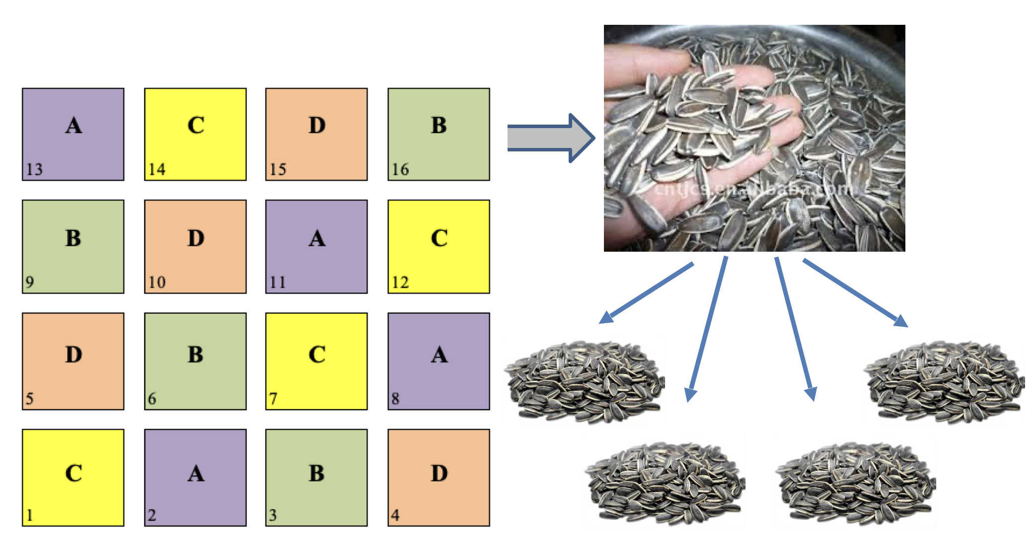
(#fig:figName13.2)An example of subsampling: from the grain yield of each plot, four samples are randomly collected and separately submitted to chemical analyses

The presence of sub-samples is a good thing, as long as true-replicates are also available. It must be clear, as we discussed in Chapter 2, that sub-samples are not to be regarded as true replicates, because the experimental treatments were not independently allocated to each of them. The four sub-samples must be regarded as sub-replicates (or pseudo-replicates) and, in absence of true-replicates, the design is to be considered as invalid.

13.2.1 Example 3: A RCBD with sub-sampling

Let’s consider a dataset from an experiment where we had 30 genotypes in three blocks and recorded the Weight of Thousand Kernels (TKW) in three sub-samples per plot. This dataset contains the ‘Sample’ variable, that is used to label the three samples in each plot. In the box below, we load the ‘TKW’ dataset from the usual repository and transform all the explanatory variables into factors.

rm(list=ls())
library(nlme)
library(emmeans)

filePath <- "https://www.casaonofri.it/_datasets/TKW.csv"
TKW <- read.csv(filePath)
TKW$Block <- factor(TKW$Block)
TKW$Genotype <- factor(TKW$Genotype)
TKW$Sample <- factor(TKW$Sample)
head(TKW)
##   Plot Block  Genotype Sample  TKW
## 1    1     1 Meridiano      1 28.6
## 2    2     1     Solex      1 33.3
## 3    3     1  Liberdur      1 22.3
## 4    4     1  Virgilio      1 28.1
## 5    5     1   PR22D40      1 26.7
## 6    6     1    Ciccio      1 34.2

It may be useful to look at the ‘naive’ analysis, that makes no distinction between true-replicates and sub-replicates and, consequently, regard the design as a RCB with 9 replicates.

# Naive analysis
mod <- lm(TKW ~ Block + Genotype, data=TKW)
anova(mod)
## Analysis of Variance Table
## 
## Response: TKW
##            Df Sum Sq Mean Sq F value    Pr(>F)    
## Block       2  110.3  55.169   7.510 0.0006875 ***
## Genotype   29 7224.7 249.129  33.913 < 2.2e-16 ***
## Residuals 238 1748.4   7.346                      
## ---
## Signif. codes:  0 '***' 0.001 '**' 0.01 '*' 0.05 '.' 0.1 ' ' 1
summary(mod)$sigma
## [1] 2.710373
pairwise <- as.data.frame(pairs(emmeans(mod, ~Genotype)))
sum(pairwise$p.value < 0.05)
## [1] 225

We see that the Root Mean Square Error is 2.71, the F test for the genotypes is highly significant and there are 225 significant pairwise comparisons among the 30 genotypes.

13.2.1.1 Model definition

The above analysis is simple, but it is also terribly wrong. By putting true-replicates and pseudo-replicates on an equal footing, we have forgotten that the 270 observations are grouped by plot and that the observations in the same plot are more alike than the observations in different plots, because they share the same ‘origin’. In other words, the observations in each plot are correlated and, therefore, the basic assumption of independence of residuals is broken. Furthermore, we pretend a higher degree of precision then we actually have: the three sub-samples are correlated and they do not contribute three full pieces of information.

A fully correct model must make the distinction between replicates and sub-replicates, by including an extra-term for the plots, that are the ‘grouping’ units:

\[ Y_{ijks} = \mu + \alpha_i + \beta_j + \gamma_{k} + \varepsilon_{s}\]

In the above model, \(Y\) is the thousand kernel weight for the i^th genotype, j^th block, k^th plot and s^th sub-sample, \(\alpha\) is the effect of the i^th genotype, \(\beta\) is the effect of the j^th block, \(\gamma\) is the effect of the the k^th plot and \(\varepsilon\) is the effect of the s^th subsample. The presence of the \(\gamma\) element accounts for the the plot-to-plot differences, so that the independence of model residuals is restored.

Obviously, the difference between plots (for a given genotype and block) must be regarded as purely random, as well as the difference between subplots, within each plot. Consequently, this is a mixed model: the two variance components are \(\sigma^2_p\) and \(\sigma^2_e\) and we see that the second one is much smaller, as it does not contain some important sources of experimental error, such as the variability due to the soil, or to the cropping practices. Obviously the first component should be given the proper weight when building the correct error term to test for the genotypes.

13.2.1.2 Model fitting with R

We can fit this mixed model by using the lmer() function in the lme4 package.

# Mixed model fit
mod.mix <- lmer(TKW ~ Block + Genotype + (1|Plot), data=TKW)
print(VarCorr(mod.mix), comp = "Variance")
##  Groups   Name        Variance
##  Plot     (Intercept) 8.89201 
##  Residual             0.84526
anova(mod.mix, ddf = "Kenward-Roger")
## Type III Analysis of Variance Table with Kenward-Roger's method
##           Sum Sq Mean Sq NumDF DenDF F value    Pr(>F)    
## Block      3.389  1.6944     2    58  2.0046    0.1439    
## Genotype 221.892  7.6515    29    58  9.0522 9.944e-13 ***
## ---
## Signif. codes:  0 '***' 0.001 '**' 0.01 '*' 0.05 '.' 0.1 ' ' 1
pairwise <- as.data.frame(pairs(emmeans(mod.mix, ~Genotype)))
sum(pairwise$p.value < 0.05)
## [1] 91

We do not show the results of pairwise comparisons for the sake of brevity; however, we point out that there are several differences with respect to the previous ‘naive’ fit:

1. in the ‘naive’ model, we have only one estimate for \(\sigma^2\), that is 7.346 with 238 DF. In this case the correct term to test for the genotype effect is \(\sigma^2_p\), that is equal to 8.892 with 58 DF. Clearly, the naive analysis strongly overestimates the number of DF: the observations taken in the same plot are correlated and they do not contribute full information.
2. The RMSE for the mixed model is equal to 2.98 and it is higher than that from the ‘naive’ fit. The variability within plots is much smaller.
3. The number of significant pairwise comparisons between genotypes has dropped to 91.

13.2.1.3 A simpler alternative

We strongly recommend the previous method of data analysis, but, whenever the number of sub-samples is the same for all plots, we can also reach correct results by proceeding in two-steps. In the first step, we calculate the means of sub-samples for each plot and, in the second step, we submit the plot means to ANOVA, by considering the genotype and the block as fixed factors. In the box below we can see that the results are exactly the same as with the mixed model fit.

# First step
TKWm <- aggregate(TKW ~ Block + Genotype, data = TKW, mean)

#Second step
mod2step <- lm(TKW ~ Genotype + Block, data = TKWm)
anova(mod2step)
## Analysis of Variance Table
## 
## Response: TKW
##           Df  Sum Sq Mean Sq F value    Pr(>F)    
## Genotype  29 2408.24  83.043  9.0522 9.943e-13 ***
## Block      2   36.78  18.390  2.0046    0.1439    
## Residuals 58  532.08   9.174                      
## ---
## Signif. codes:  0 '***' 0.001 '**' 0.01 '*' 0.05 '.' 0.1 ' ' 1

13.3 Repeated experiments

In Chapter 1 we mentioned that results need to be replicable and, hopefully, reproducible. The presence of true replicates ensures replicability, i.e. that the results can be reproduced in the same conditions. However, true replication does not ensure that the results are reproducible in different conditions.

For this reason, experiments should be usually repeated in different runs, sites, years or, more generally, in different environments. This is a fundamental key to scientific progress in agriculture and permits sound generalisation; otherwise, the results are specific to the conditions in which they were obtained and their scope is rather limited. Multi-year or multi-site experiments are very common, e.g., in plant breeding and they may involve wide groups of research units across countries or continents. These research units usually employ a commone core of genotypes and the same experimental design (e.g.: randomised complete blocks with 3-4 replicates), while innovative genotypes are progressively introduced in each year and the old ones tend to be abandoned.

Apart from genotype trials, all types of field experiments should be usually repeated at least in two-three different environments (sites or years) to have a minimum appraisal of the reproducibility of results. More generally, we should not underrate the importance of repeating all types of experiments, including those performed in the greenhouse or in controlled conditions, especially when we make use of sampled units from populations with a high degree of spatial or temporal variability (e.g.: seeds, plants, leaves and so on). Based on our experience, we suggest that the variability of results across different runs of the same experiment may be pretty high and, therefore, we argue that a single experiment in agriculture proves nothing.

13.3.1 A model for pooling the results

In general, each repeated experiment produces data that can be analysed on its own, by using one of the methods described in the previous chapters. However, a pooled analysis is in order, to consolidate the results over the runs and assess their reproducibility. When we pool a set of one-factor experiments, the pooled dataset becomes similar to a two-factor factorial experiment; analogously to what we have described in Chapter 11, a possible model is:

\[ y_{ijk} = \mu + \alpha_i + \beta_j + \alpha\beta_{ij} + \varepsilon_{ijk}\]

where \(y\) is the response for the i^th run, j^th treatment level and k^th replicate, \(\mu\) is the intercept (the overall mean, when the sum-to-zero constraint is adopted), \(\alpha\) is the effect of the i^th run, \(\beta\) is the effect of the j^th treatment level, \(\alpha\beta\) is the ‘treatment x run’ interaction effect and \(\varepsilon\) is the residual random effect for each observation, which we assume as normally distributed (\(\epsilon_{ijk} \sim N(0, \sigma_{\varepsilon})\))

One difference with two-factor factorial experiments is that, when we repeat experiments laid down in complete blocks, we need to add to the model the term \(\gamma_{ik}\), that is the effect of the k^th block in the i^th run. Indeed, the block effect is nested within runs, as the block levels are usually different in different runs.

Obviously, if we need to pool a set of multi-factorial experiments, the model becomes more complex and we need to include all possible interactions between the treatment factors and their combinations with the run factor. For example, if we have a set of two-factor (A and B) factorial experiments, we need to consider the following effects (in R notation): ‘A + B + A:B + A:run + B:run + A:B:run’, that is equivalent to writing ‘A * B * run’.

13.3.2 Preliminary analyses

It is always convenient to start with a preliminary evaluation of each single experiment and, afterwards, perform a pooled fit. We would suggest this process:

1. fit an ANOVA model to each experiment (as shown in previous Chapters);
2. inspect the data to assess whether we have good data for all runs. Search for possible outliers and for heteroscedasticity of within-run errors (as shown in Chapter 8);
3. if possible, fit a pooled model;
4. inspect the residuals from the pooled model, with particular reference to possible heteroscedasticy across runs.

13.3.3 Fixed or random runs?

What is peculiar about repeated experiments is that we always need to take a decision about the nature of the run effect, whether it is ‘fixed’ or ‘random’. Such decision is specific to each experiment and it is up to the researcher, who should give solid reasons to support it. It is not easy to give suggestions; as the rule of thumb, whenever the experiment is repeated in a small number of runs (e.g. 2 or 3), we could think of taking the run effect as fixed. Indeed, a reliable estimation of variance components requires that the number of levels for the random factor is sufficiently high (roughly 4, at least).

With field experiments repeated in a relatively high number of years/locations, the year effect seems to be reasonably random. Indeed, although the years are not sampled (we cannot sample years, we can only take them in the same order as they come), the effects they produce are not repeatable and they are clearly of random nature. On the other hand, the location effect is more dubious: sometimes, the locations are selected on purpose and they are interesting on themselves, so that the location effect is fixed. In other instances, locations are sampled to represent a macro-environment and, therefore, their effect is random.

Selecting the run factor as fixed or random has an impact on the results of data analyses, as we will see in the following two examples.

13.3.4 Example 4: a seed germination experiment in two runs

The germination of three genotypes of oilseed rape was assessed by a greenhouse bioassay with six replicated Petri dishes per genotype (18 dishes in total). Fifty seeds were put in each dish and the number of germinated seeds was counted after 15 days and expressed as the Final Proportion of Germinated seeds (FGP). The assay was repeated twice in slightly different conditions, because the environmental parameters in the greenhouse were not under full control. The results are online available as the ‘FGP_rape.csv’ text file and they can be loaded by using the code below.

fileName <- "https://www.casaonofri.it/_datasets/FGP_rape.csv"
dataset <- read.csv(fileName)
dataset[,1:5] <- lapply(dataset[,1:5], factor)

Preliminarily, in order to fit the ANOVA models to each single run, we can very much simplify the coding by using the ‘by()’ and ‘lapply()’ functions. The first one, operates on subsets of the selected dataset, according to a classification variable (the run, in this case) and produces a list with the resulting model objects. ‘Lapply()’ applies a function to all elements in a list and, in the following code, we used it to perform a Levene’s test for homoscedasticity and a Shapiro-Wilks test for normality.

library(MASS)
lmFits <- by(dataset, dataset$Run,  
      function(df) lm(FGP ~ Genotype, data = df) )

# Check for within-experiments homoscedasticity/normality
lapply(lmFits, function(mods) car::leveneTest(mods))
## $`1`
## Levene's Test for Homogeneity of Variance (center = median)
##       Df F value Pr(>F)
## group  2  2.6856 0.1007
##       15               
## 
## $`2`
## Levene's Test for Homogeneity of Variance (center = median)
##       Df F value Pr(>F)
## group  2   1.222 0.3224
##       15
lapply(lmFits, function(mods) shapiro.test(residuals(mods)))
## $`1`
## 
##  Shapiro-Wilk normality test
## 
## data:  residuals(mods)
## W = 0.94221, p-value = 0.316
## 
## 
## $`2`
## 
##  Shapiro-Wilk normality test
## 
## data:  residuals(mods)
## W = 0.93291, p-value = 0.2184
# Variance partitioning
lapply(lmFits, function(mods) anova(mods))
## $`1`
## Analysis of Variance Table
## 
## Response: FGP
##           Df   Sum Sq   Mean Sq F value   Pr(>F)   
## Genotype   2 0.033011 0.0165056  8.1353 0.004047 **
## Residuals 15 0.030433 0.0020289                    
## ---
## Signif. codes:  0 '***' 0.001 '**' 0.01 '*' 0.05 '.' 0.1 ' ' 1
## 
## $`2`
## Analysis of Variance Table
## 
## Response: FGP
##           Df   Sum Sq   Mean Sq F value    Pr(>F)    
## Genotype   2 0.042544 0.0212722   22.34 3.177e-05 ***
## Residuals 15 0.014283 0.0009522                      
## ---
## Signif. codes:  0 '***' 0.001 '**' 0.01 '*' 0.05 '.' 0.1 ' ' 1

The previous results demonstrate that the basic assumptions for linear models are reasonably met and that the two assays produced significant results, in relation to the genotype effect. Therefore, we move on to pooling the data from the two experiments.

13.3.4.1 Model fitting with R

As we have only two runs in similar (not totally equivalent) environmental conditions, it might be appropriate to regard the ‘run’ effect as fixed: are the results comparable across these two specific runs? Consequently, we have a fixed effects model, that can be fitted by using the lm() function, as shown in the box below:

mod <- lm(FGP ~ Genotype * Run, data = dataset)

Before looking at the results, we need to check the whole model and, in particular, we need to check that the residuals from the different runs have homogeneous variances. We do so by using a likelihood approach that is available in the ‘check.hom()’ function in the aomisc package.

library(nlme)
library(aomisc)
## Loading required package: drc
## Loading required package: drcData
## 
## 'drc' has been loaded.
## Please cite R and 'drc' if used for a publication,
## for references type 'citation()' and 'citation('drc')'.
## 
## Attaching package: 'drc'
## The following objects are masked from 'package:stats':
## 
##     gaussian, getInitial
## Loading required package: plyr
## --------------------------------------------------------------------
## You have loaded plyr after dplyr - this is likely to cause problems.
## If you need functions from both plyr and dplyr, please load plyr first, then dplyr:
## library(plyr); library(dplyr)
## --------------------------------------------------------------------
## 
## Attaching package: 'plyr'
## The following objects are masked from 'package:reshape':
## 
##     rename, round_any
## The following objects are masked from 'package:dplyr':
## 
##     arrange, count, desc, failwith, id, mutate, rename,
##     summarise, summarize
## Loading required package: car
## Loading required package: carData
## 
## Attaching package: 'car'
## The following object is masked from 'package:dplyr':
## 
##     recode
## Loading required package: multcompView
## Registered S3 method overwritten by 'aomisc':
##   method   from
##   plot.nls nlme
check <- check.hom(mod, Run)
check$aovtable
##      Model df       AIC       BIC   logLik   Test  L.Ratio p-value
## mod1     1  7 -85.37132 -75.56294 49.68566                        
## mod2     2  8 -85.46782 -74.25824 50.73391 1 vs 2 2.096495  0.1476

We see that the null hypothesis of no heteroscedasticity of residuals across runs can be accepted and, therefore, we inspect the ANOVA table for the model fit.

anova(mod)
## Analysis of Variance Table
## 
## Response: FGP
##              Df   Sum Sq  Mean Sq F value    Pr(>F)    
## Genotype      2 0.074289 0.037144 24.9199 4.203e-07 ***
## Run           1 0.003025 0.003025  2.0294    0.1646    
## Genotype:Run  2 0.001267 0.000633  0.4249    0.6577    
## Residuals    30 0.044717 0.001491                      
## ---
## Signif. codes:  0 '***' 0.001 '**' 0.01 '*' 0.05 '.' 0.1 ' ' 1

In general, inspecting the ANOVA table gives us the possibility of veryifing to what extent the results of the first run were reproducible in the second run. When the run effect is fixed, the interpretation is very much like that for a two-factor factorial experiment; indeed, we can encounter the following situations:

1. the ‘run by treatment’ interaction is significant. In this case, we ought to conclude that the effects of treatment levels and, possibly, their ranking, changed in each run. Consequently, the results of our experiment were not reproducible and it makes no sense to try to pool them: we should only display and compare the means of treatment levels within each environment/run.
2. The interaction is not significant, but the run main effect is significant. We ought to conclude that the treatment effect and the run effect were independent and additive; consequently, the means for treatment levels changed across repetitions, but treatment effects were fully reproducible. It is up to the researcher to decide whether it is appropriate and meaningful to calculate and display the means for treatment levels.
3. Neither the interaction, nor the run main effects are significant. The results of the repeated experiments are fully reproducible and it is usually appropriate to report only the means for treatment levels.

For our example, we see that the ‘run’ and ‘run by treatment’ effects are not significant, which means that the results are fully reproducible. Therefore, we are allowed to pool the two runs and compare the genotypes across runs, by using the usual ‘emmeans()’ function in the ‘emmeans()’ package.

library(emmeans)
library(multcomp)
## Loading required package: mvtnorm
## Loading required package: survival
## Loading required package: TH.data
## 
## Attaching package: 'TH.data'
## The following object is masked from 'package:MASS':
## 
##     geyser
cld(emmeans(mod, ~ Genotype), Letters = LETTERS)
## NOTE: Results may be misleading due to involvement in interactions
##  Genotype emmean     SE df lower.CL upper.CL .group
##  C         0.781 0.0111 30    0.758    0.804  A    
##  A         0.871 0.0111 30    0.848    0.894   B   
##  B         0.882 0.0111 30    0.860    0.905   B   
## 
## Results are averaged over the levels of: Run 
## Confidence level used: 0.95 
## P value adjustment: tukey method for comparing a family of 3 estimates 
## significance level used: alpha = 0.05 
## NOTE: If two or more means share the same grouping symbol,
##       then we cannot show them to be different.
##       But we also did not show them to be the same.

13.3.5 Example 5: a multi-year winter wheat experiment

Let’s consider a field experiment to compare eight winter wheat genotypes, laid down in complete blocks, with three replicates. The experiment was repeated in seven years; please, note that part of this dataset has already been used for the example at Chapter 10. The response variable is the yield, in tons per hectare.

rm(list = ls())
fileName <- "https://www.casaonofri.it/_datasets/WinterWheat.csv"
WinterWheat <- read.csv(fileName)
WinterWheat$Block <- as.factor(WinterWheat$Block)
WinterWheat$Year <- as.factor(WinterWheat$Year)
head(WinterWheat, 8)
##   Plot Block Genotype Yield Year
## 1    2     1 COLOSSEO  6.73 1996
## 2  110     2 COLOSSEO  6.96 1996
## 3  181     3 COLOSSEO  5.35 1996
## 4    2     1 COLOSSEO  6.26 1997
## 5  110     2 COLOSSEO  7.01 1997
## 6  181     3 COLOSSEO  6.11 1997
## 7   17     1 COLOSSEO  6.75 1998
## 8  110     2 COLOSSEO  6.82 1998

For the sake of simplicity and brevity, we disregard the preliminary analyses of each single experiment, which could be performed by using the same code as given for the previous example.

13.3.5.1 Model fitting with R

We have a relatively high number of years and, as we explained, the year effect is intrinsically of random nature, because it is ‘not repeatable’. Therefore, we take the year effect as random and we assume that it is guassian, with mean equal 0 and standard deviation equal to \(\sigma_E\):

\[\alpha_i \sim N(0, \sigma_E)\]

The corresponding variance (\(\sigma^2_E\)) is the so-called ‘variance component’ for the year effect. If the year is random, also the ‘genotype x year’ and the ‘block|year’ effects are random and they are defined as:

\[\alpha\beta_{i,j} \sim N(0, \sigma_{GE})\]

\[\gamma_{i,k} \sim N(0, \sigma_{EB})\]

Before fitting a mixed model, we decide to fit a fixed model, for a preliminary evaluation of model residuals and to compare with the results of a mixed model fit.

modfix <- lm(Yield ~ Year/Block + Genotype * Year,
             data = WinterWheat)
check <- check.hom(modfix, Year)
check$aovtable
##      Model df      AIC      BIC    logLik   Test  L.Ratio p-value
## mod1     1 71 316.3539 499.8865 -87.17693                        
## mod2     2 77 319.4480 518.4904 -82.72398 1 vs 2 8.905903  0.1789
anova(modfix)
## Analysis of Variance Table
## 
## Response: Yield
##               Df  Sum Sq Mean Sq  F value    Pr(>F)    
## Year           6 159.279 26.5466 178.3996 < 2.2e-16 ***
## Genotype       7  11.544  1.6491  11.0824 2.978e-10 ***
## Year:Block    14   3.922  0.2801   1.8826   0.03738 *  
## Year:Genotype 42  27.713  0.6598   4.4342 6.779e-10 ***
## Residuals     98  14.583  0.1488                       
## ---
## Signif. codes:  0 '***' 0.001 '**' 0.01 '*' 0.05 '.' 0.1 ' ' 1

The previous box suggests that there is no problem with the heteroscedasticity of model residuals across years. The ‘genotype by year’ interaction is significant and, therefore, if the ‘year effect’ is taken as fixed, we could only compare genotypes within years, which is rather meaningless, due to the unreplicability of the year effect. Therefore, it is much more useful to switch to a mixed model fit.

This latter can be fitted by using the lmer() function, as shown below:

mod <- lmer(Yield ~ (1|Year) + (1|Year:Block) + Genotype +
               (1|Year:Genotype),
             data = WinterWheat)

First of all, we inspect the estimates of variance components, because they represent the sources of random variability. With balanced data (as in this case), these variance components could also be obtained by using the method of moments, starting from the ANOVA table from a fixed model fit:

\[\sigma^2_{\varepsilon} = MS_{\varepsilon}\]

\[ \sigma^2_{GE} = \frac{MS_{GE} - \sigma^2_{\varepsilon}}{n_B} = \frac{0.6598 - 0.1488}{3} = 0.1703\]

\[ \sigma^2_{EB} = \frac{MS_{EB} - \sigma^2_{\varepsilon}}{n_G} = \frac{0.2801 - 0.1488}{8} = 0.0164\]

\[ \sigma^2_{E} = \frac{MS_E - 8 \, \sigma^2_{EB} - 3 \, \sigma^2_{GE} - \sigma^2_{\varepsilon}}{n_{GB}} = \]

\[ = \frac{26.55 - 8 \times 0.0164 - 3 \times 0.1703 - 0.1488}{24} = 1.073\]

where \(n_B\), \(n_G\) and \(n_{GB}\) are, respectively, the number of blocks, the number of genotypes and the number of ‘genotype by block’ combinations, while \(\textrm{MS}_{\varepsilon}\), \(\textrm{MS}_E\), \(\textrm{MS}_{EB}\) and \(\textrm{MS}_{GE}\) are the mean squares from a fixed effect fit, respectively, for the residual error, the years, the blocks within years and the genotype by year interaction. However, the REstricted Maximum Likelihood (REML) estimates provided by the ‘lmer()’ function are simpler to obtain, also with unbalance data.

# Variance components
print( VarCorr(mod), comp=c("Variance", "Std.Dev.") )
##  Groups        Name        Variance Std.Dev.
##  Year:Genotype (Intercept) 0.170341 0.41272 
##  Year:Block    (Intercept) 0.016418 0.12813 
##  Year          (Intercept) 1.073146 1.03593 
##  Residual                  0.148804 0.38575

The variance component estimates show that the overall yield variability is mainly due to the year effect (year-to-year variability: \(\sigma_E = 1.04\)), which was the same for all genotypes. This source of variability impacts on genotype mean yields (which changes depending on the year), but it does not impact on genotype effects and differences. Another important source of variability is the genotype-by-year interaction (\(\sigma_{GE} = 0.41\)), which is additional to the year-to-year variability and it is highly specific to each genotype. It impacts on genotype mean, but it also impact on genotype effects (and differences), that change depending on the years. The within year plot-to-plot variability is smaller (\(\sigma = 0.39\)), although it is clear that it impacts on genotype means, effects and differences. Last, block-to-block variability (\(\sigma_{EB} = 0.13\)) is the smallest component and, similarly to year-to-year variability, it is the same for all genotypes and it impacts only on their mean value across blocks.

# ANOVA table
anova(mod)
## Type III Analysis of Variance Table with Satterthwaite's method
##          Sum Sq Mean Sq NumDF DenDF F value  Pr(>F)  
## Genotype 2.6033  0.3719     7    42  2.4993 0.03058 *
## ---
## Signif. codes:  0 '***' 0.001 '**' 0.01 '*' 0.05 '.' 0.1 ' ' 1

The ANOVA table only includes the genotype effect, because all other effects are random and it makes no sense to test for the existence of a significant difference between the means for the different factor levels. We see that the F ratio for the genotype effect is smaller than that from a fixed model fit, because it needs to consider, at the denominator, all the main sources of variability that can impact on the genotype effects (i.e.: plot-to-plot variability and the genotype-by-year interaction). In particular, the F ratio is obtained as:

\[F = \frac{MS_G}{n_B \times \sigma^2_{GE} + \sigma^2_{\varepsilon}} = \frac{MS_G}{MS_{GE}} = \frac{1.6491}{0.6598} = 2.499\]

When the year effect is random, we can always consider and compare the means of genotypes across years and we are not restrained by a significant genotype-by-year interaction. However, SEMs and SEDs are usually higher than those from a fixed model fit, because they have to consider all possible sources of variability. In particular, with a fixed effects model, the standard errors for the genotype means is (\(r\) is the number of replicates and \(n_e\) is the number of environments):

\[SEM_f = \sqrt{ \frac{\sigma^2}{r\,n_e} } = \sqrt{ \frac{0.1488}{3 \cdot 7}} = 0.0842\]

With mixed models, the SEM is calculated by considering all sources of random variability:

\[SEM_m = \sqrt \frac{r \, \sigma^2_E + \sigma^2_{EB} + r \sigma^2_{GE} + \sigma^2 }{re} = \sqrt \frac{3 \cdot 1.073 + 0.016 + 3 \cdot 0.170 + 0.1488 }{3 \cdot 7} = 0.431\]

Likewise, the Standard Error of a Difference (SED), for the mixed model, is calculated by considering the plot-to-plot variability and the genotype-by-environment variability, while the year-to-year variability and the block-to-block variability are not considered, because they impact on all the means in the same way and, therefore, they do not impact on the differences. The expressions are:

\[SED_f = \sqrt{2 \, \frac{\sigma^2}{r \, n_e} } \quad \quad SED_m = \sqrt {2 \, \frac{r \, \sigma^2_{ge} + \sigma^2 }{r \, n_e} }\]

Marginal means and significance letters can be easily obtained as shown in previous examples and chapters:

cld(emmeans(mod, ~Genotype), Letters = letters,
    adjust = "none")
##  Genotype emmean    SE   df lower.CL upper.CL .group
##  SIMETO     5.93 0.431 8.23     4.94     6.91  a    
##  CRESO      5.97 0.431 8.23     4.99     6.96  a    
##  GRAZIA     6.08 0.431 8.23     5.09     7.07  a    
##  SANCARLO   6.22 0.431 8.23     5.23     7.21  ab   
##  SOLEX      6.23 0.431 8.23     5.24     7.22  ab   
##  COLOSSEO   6.41 0.431 8.23     5.43     7.40  ab   
##  DUILIO     6.59 0.431 8.23     5.60     7.58   b   
##  IRIDE      6.70 0.431 8.23     5.71     7.68   b   
## 
## Degrees-of-freedom method: kenward-roger 
## Confidence level used: 0.95 
## significance level used: alpha = 0.05 
## NOTE: If two or more means share the same grouping symbol,
##       then we cannot show them to be different.
##       But we also did not show them to be the same.

We see that the correction of multiplicity and the need to consider all sources of random yield variability, does not permit to prove the existence of any significant difference between genotypes.

13.4 Repeated measures in perennial crops

With perennial crops measures are taken repeatedly in the same plots across years. For this reason, even though the dataset looks very much like that for the winter wheat experiment repeated in several years, it must be analysed in a totally different manner.

In particular, we should not neglect that, in contrast to the winter wheat example, the observations are grouped within the same plots and, therefore, they are not independent, because the observations taken on the same plot are more alike than observations taken on different plots. We have seen a similar situation with the subsampling experiment given before, with an important difference: while subsamples were taken at random within each plot, repeated measures may not be sampled at random, they may be specifically taken to evaluate the yield in different moments of plant life.

13.4.1 Example 5: genotype experiment with lucerne

Let’s consider the dataset below, that refers to the yield of lucerne genotypes in three consecutive years, taken from the same plots in a single experiment lasting for three years. In the box below we load the data and make the necessary transformations. We also build a new variable to uniquely identify each plot, which is easy, considering that yield values taken for the same genotype in the same block must have been taken in the same plot.

filePath <- "https://www.casaonofri.it/_datasets/alfalfa3years.csv"
dataset <- read.csv(filePath)
dataset$Block <- factor(dataset$Block)
dataset$Genotype <- factor(dataset$Genotype)
dataset$Year <- factor(dataset$Year)
head(dataset)
##   Block Genotype Year     Yield
## 1     1 4cascine 2006  6.631775
## 2     2 4cascine 2006  6.705397
## 3     3 4cascine 2006  6.499588
## 4     4 4cascine 2006  7.087686
## 5     1 4cascine 2007 14.964927
## 6     2 4cascine 2007 13.584865
# Reference the plots
dataset$Plot <- dataset$Block:dataset$Genotype

13.4.1.1 Model definition

For repeated measures designs, models can be built by using the rules in Piepho et al. (2004):

1. Consider one single year and build the treatment model
2. Consider one single year and build the block model
3. Include the year factor into the model and combine the year with all the effects in the treatment model, by crossing or nesting as appropriate.
4. Consider that the ‘plot’ factor in the block model references the randomisation units, i.e. those units which received the the genotypes by a randomisation process. Assign to this plot factor a random effect.
5. Excluding the terms for randomisation units, nest the year in all the other terms in the block model.
6. Combine random effects for randomisation units with the repeated factor, by using the colon operator, in order to derive the correct error terms to accommodate correlation structures.

The models at the different steps are as follows (with R notation):

1. treatment model: YIELD ~ GENOTYPE
2. block model: YIELD ~ BLOCK + BLOCK:PLOT
3. treatment model: YIELD ~ GENOTYPE * YEAR
4. block model: YIELD ~ BLOCK + (1|BLOCK:PLOT)
5. block model: YIELD ~ BLOCK + BLOCK:YEAR + (1|BLOCK:PLOT)
6. block model: YIELD ~ BLOCK + BLOCK:YEAR + (1|BLOCK:PLOT) + (1|BLOCK:PLOT:YEAR)

In this case, considering that lucerne lasts, on average, for three years and follows a specific pattern of yield across these three years, we decided to take the block, year and genotype effects as fixed; therefore, the final model, with R notation, is:

YIELD ~ BLOCK + BLOCK:YEAR + GENOTYPE * YEAR + (1|BLOCK:PLOT) + (1|BLOCK:PLOT:YEAR)

where the last term does not need to be fitted in R, as it is the residual term, that is fitted by default. The resulting analysis (with ‘lmer’) is:

mod <- lmer(Yield ~ Block + Block:Year + Genotype*Year +
            (1|Plot:Block),
           data = dataset)
anova(mod)
## Type III Analysis of Variance Table with Satterthwaite's method
##                Sum Sq Mean Sq NumDF DenDF   F value    Pr(>F)    
## Block            3.96    1.32     3    57    2.1389  0.105316    
## Genotype        54.00    2.84    19    57    4.6024  3.75e-06 ***
## Year          2602.53 1301.27     2   114 2107.3223 < 2.2e-16 ***
## Block:Year      14.14    2.36     6   114    3.8176  0.001667 ** 
## Year:Genotype   31.83    0.84    38   114    1.3563  0.111546    
## ---
## Signif. codes:  0 '***' 0.001 '**' 0.01 '*' 0.05 '.' 0.1 ' ' 1
emmeans(mod, ~Genotype)
## NOTE: Results may be misleading due to involvement in interactions
##  Genotype          emmean    SE df lower.CL upper.CL
##  4cascine           11.59 0.315 57    10.96     12.2
##  casalina           12.46 0.315 57    11.83     13.1
##  classe             11.59 0.315 57    10.96     12.2
##  costanza            9.89 0.315 57     9.26     10.5
##  dimitra            11.75 0.315 57    11.12     12.4
##  FDL0101            12.22 0.315 57    11.59     12.9
##  garisenda          11.76 0.315 57    11.13     12.4
##  LaBellaCampagnola  12.17 0.315 57    11.54     12.8
##  LaTorre            11.36 0.315 57    10.73     12.0
##  linfa              11.23 0.315 57    10.60     11.9
##  marina             11.76 0.315 57    11.13     12.4
##  Palladiana         10.89 0.315 57    10.26     11.5
##  PicenaGR           12.12 0.315 57    11.49     12.8
##  PR56S82            11.56 0.315 57    10.93     12.2
##  PR57Q53            11.70 0.315 57    11.07     12.3
##  prosementi         11.79 0.315 57    11.15     12.4
##  RivieraVicentina    9.98 0.315 57     9.35     10.6
##  robot              12.11 0.315 57    11.48     12.7
##  Selene             12.11 0.315 57    11.48     12.7
##  Zenith             11.94 0.315 57    11.31     12.6
## 
## Results are averaged over the levels of: Block, Year 
## Degrees-of-freedom method: kenward-roger 
## Confidence level used: 0.95

We see that the ‘genotype x year’ interaction is not significant, so that we can proceed to comparing the means of genotypes across years, which can be done with the ‘emmeans()’ function in the usual fashion.

It may be useful to compare this analysis with a ‘naive’ (and wrong) analysis that neglects the repeated measures (i.e., that neglects the ‘plot’ random effect). Wee see big differences and, especially, we see that the SEs for genotype means are much higher in the correct analysis.

mod2 <- lm(Yield ~ Year/Block + Genotype*Year, 
           data = dataset)
anova(mod2)
## Analysis of Variance Table
## 
## Response: Yield
##                Df  Sum Sq Mean Sq   F value    Pr(>F)    
## Year            2 2602.53 1301.27 1608.2407 < 2.2e-16 ***
## Genotype       19  104.27    5.49    6.7824 4.256e-13 ***
## Year:Block      9   21.80    2.42    2.9930  0.002449 ** 
## Year:Genotype  38   31.83    0.84    1.0351  0.424687    
## Residuals     171  138.36    0.81                        
## ---
## Signif. codes:  0 '***' 0.001 '**' 0.01 '*' 0.05 '.' 0.1 ' ' 1
emmeans(mod2, ~Genotype)
## NOTE: A nesting structure was detected in the fitted model:
##     Block %in% Year
## NOTE: Results may be misleading due to involvement in interactions
##  Genotype          emmean   SE  df lower.CL upper.CL
##  4cascine           11.59 0.26 171    11.07     12.1
##  casalina           12.46 0.26 171    11.94     13.0
##  classe             11.59 0.26 171    11.08     12.1
##  costanza            9.89 0.26 171     9.38     10.4
##  dimitra            11.75 0.26 171    11.24     12.3
##  FDL0101            12.22 0.26 171    11.71     12.7
##  garisenda          11.76 0.26 171    11.24     12.3
##  LaBellaCampagnola  12.17 0.26 171    11.66     12.7
##  LaTorre            11.36 0.26 171    10.84     11.9
##  linfa              11.23 0.26 171    10.72     11.7
##  marina             11.76 0.26 171    11.25     12.3
##  Palladiana         10.89 0.26 171    10.38     11.4
##  PicenaGR           12.12 0.26 171    11.61     12.6
##  PR56S82            11.56 0.26 171    11.05     12.1
##  PR57Q53            11.70 0.26 171    11.19     12.2
##  prosementi         11.79 0.26 171    11.27     12.3
##  RivieraVicentina    9.98 0.26 171     9.47     10.5
##  robot              12.11 0.26 171    11.59     12.6
##  Selene             12.11 0.26 171    11.60     12.6
##  Zenith             11.94 0.26 171    11.42     12.5
## 
## Results are averaged over the levels of: Block, Year 
## Confidence level used: 0.95

We just want to conclude by saying that the above mixed model analyses regards the design as a sort of ‘split-plot in time’ and it is not necessarily correct, as it assumes that the within-plot correlation is the same for all pairs of observations, regardless of their distance in time. Further analyses might be necessary to assess whether serial correlation structures are necessary, although such an aspect is far beyond the scope of this book.

13.5 Further readings

1. Annichiarico, P., 2002. Genotype x Environment Interactions - Challenges and Opportunities for Plant Breeding and Cultivar Recommendations. FAO, 1, 1-115 (This is on-line available. Just make a google search!)
2. Bates, D., Mächler, M., Bolker, B., Walker, S., 2015. Fitting Linear Mixed-Effects Models Using lme4. Journal of Statistical Software 67. https://doi.org/10.18637/jss.v067.i01
3. Gałecki, A., Burzykowski, T., 2013. Linear mixed-effects models using R: a step-by-step approach. Springer, Berlin.
4. Kuznetsova, A., Brockhoff, P.B., Christensen, H.B., 2017. lmerTest Package: Tests in Linear Mixed Effects Models. Journal of Statistical Software 82, 1–26.
5. Piepho, H.-P., Büchse, A., Richter, C., 2004. A Mixed Modelling Approach for Randomized Experiments with Repeated Measures. Journal of Agronomy and Crop Science 190, 230–247.