This is a follow-up post. If you are interested in other posts of this series, please go to: https://www.statforbiology.com/tags/drcte/. All these posts exapand on a paper that we have recently published in the Journal ‘Weed Science’; please follow this link to the paper.
Reshaping time-to-event data
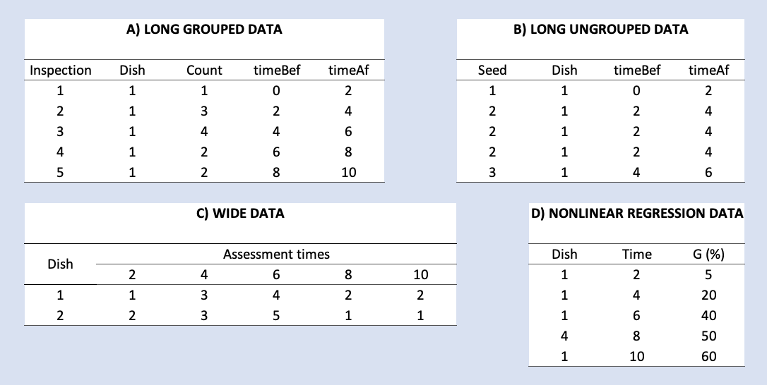
The first thing we should consider before working through this tutorial is the structure of germination/emergence data. To our experience, seed scientists are used to storing their datasets in several formats, that may not be immediately usable with the ‘drcte’ and ‘drc’ packages, which this tutorial is built upon. The figure below shows some of the possible formats that I have often encountered in my consulting work.
{width=90%}
Both the ‘drcte’ and ‘drc’ packages require that the data is stored in LONG GROUPED format, as shown in the figure above (panel A, top left). Each row represents a time interval, the columns ‘timeBef’ and ‘timeAf’ represent the beginning and ending of the interval, while the column ‘count’ represents the seeds that germinated/emerged during that interval of time. Other columns may be needed, to represent, e.g., the randomisation unit (e.g., Petri dish) within which the count was made and the experimental treatment level that was allocated to that unit.
Apart from the LONG GROUPED format, other time-to-event packages, such as ‘survival’ (Therneau, 2021) or ‘interval’ (Fay and Shaw, 2010) require a different data format, which could be named as LONG UNGROUPED (Figure above, panel B, top right). In this format, each row represents a seed, while the columns ‘timeBef’ and ‘timeAf’ represent the beginning and ending of the interval during which that seed germinated/emerged. The column ‘count’ is not necessary, while other columns may be necessary, as for the LONG GROUPED format. Apart from the above mentioned ‘survival’ and ‘interval’ packages, this format is also compatible with the ‘drcte’ package.
Both the GROUPED and UNGROUPED formats have two basic advantages: (i) they can be used with all types of time-to-event data and (ii) they obey to the principles of tidy data (Wickham, 2016). However, to my experience, seed scientists often use other formats, such as the WIDE format (Figure above, panel C, bottom left) or the NONLINEAR REGRESSION format (Figure above, panel D, bottom right), which need to be preliminary transformed into one of the LONG GROUPED or LONG UNGROUPED formats.
In order to ease the transition from traditional methods of data analysis to time-to-event methods, we decided to develop a couple of service functions that can be used to reshape the data to a format that is more suitable for time-to-event analyses. Let’s see how to do this by using a ‘real-life’ example.
Motivating example
Seeds of L. ornithopodioides were collected from natural populations, at three different maturation stages, i.e. at 27 Days After Anthesis (DAA), when seeds were still green (Stage A), at 35 DAA, when seeds were brown and soft (Stage B) and at 41 DAA, when seeds were brown and moderately hard (Stage C). Germination assays were performed by placing four replicates of 25 seeds on filter paper (Whatman no. 3) in 9-cm diameter Petri dishes, in the dark and at a constant temperature of 20°C. The filter paper was initially moistened with 5 mL of distilled water and replenished as needed during the assay. Germinated seeds were counted daily over 15 days and removed from the Petri dishes. This dataset is a subset of a bigger dataset, aimed at assessing the time when the hard coat imposes dormancy in seeds of different legume species (Gresta et al., 2011).
The authors of the above study sent me the above dataset in WIDE format, where the rows represented each Petri dish and the columns represented all information about each dish, including the counts of germinated seeds, which were listed in different columns. The dataset is shown in the table below and it is available as the ‘lotusOr’ dataframe in the ‘drcte’ package.
library(drcte)
data(lotusOr)
print(lotusOr, row.names = F)
##  Stage Dish 1  2 3 4 5 6 7 8 9 10 11 12 13 14 15
##      A    1 0  0 0 0 0 1 2 1 1  1  3  1  1  4  2
##      A    2 0  0 0 0 0 1 1 1 1  2  1  2  3  1  1
##      A    3 0  0 0 0 0 3 4 4 3  1  2  1  1  0  1
##      A    4 0  0 0 0 0 1 3 1 2  1  2  1  3  1  1
##      B    5 0  0 0 4 1 2 1 1 0  1  2  2  3  2  1
##      B    6 0  0 0 4 2 2 1 0 1  1  3  4  3  4  0
##      B    7 0  0 0 4 0 4 1 2 1  1  3  3  2  2  0
##      B    8 0  0 0 4 3 2 2 3 1  1  1  1  1  0  0
##      C    9 1 10 1 2 1 2 3 2 0  0  0  0  1  0  0
##      C   10 1 10 4 1 4 0 1 1 0  0  0  0  1  0  1
##      C   11 1 11 5 1 2 2 1 0 1  0  0  1  0  0  0
##      C   12 0 16 1 2 2 1 1 0 0  1  0  0  0  1  0
The WIDE format is handy for swift calculations with a spreadsheet, but, in general, it is not ok, as: (1) it does not obey to the principle of tidy data (Wickham, 2016); (2) it is not generally efficient and it cannot be used with a set of germination assays with different monitoring schedules. Therefore, facing a dataset in the WIDE format, we need to reshape it into a LONG format.
Transforming from WIDE to LONG GROUPED
For such a reshaping, we could use one of the available R functions, such us pivot_longer() in the ‘tidyverse’ or melt() in the ‘reshape’ package. However, when reshaping the data, it is also useful to make e few transformations, such as producing cumulative counts and proportions, that might be useful to plot graphs, or for other purposes. Therefore, we developed the melt_te() function; let’s look at its usage, in the box below.
datasetG <- melt_te(lotusOr, count_cols = 3:17, treat_cols = Stage,
                   monitimes = 1:15, n.subjects = rep(25,12))
head(datasetG, 16)
##    Stage Units timeBef timeAf count nCum propCum
## 1      A     1       0      1     0    0    0.00
## 2      A     1       1      2     0    0    0.00
## 3      A     1       2      3     0    0    0.00
## 4      A     1       3      4     0    0    0.00
## 5      A     1       4      5     0    0    0.00
## 6      A     1       5      6     1    1    0.04
## 7      A     1       6      7     2    3    0.12
## 8      A     1       7      8     1    4    0.16
## 9      A     1       8      9     1    5    0.20
## 10     A     1       9     10     1    6    0.24
## 11     A     1      10     11     3    9    0.36
## 12     A     1      11     12     1   10    0.40
## 13     A     1      12     13     1   11    0.44
## 14     A     1      13     14     4   15    0.60
## 15     A     1      14     15     2   17    0.68
## 16     A     1      15    Inf     8   NA      NA
The melt_te() function requires the following arguments:
- data: the original dataframe
- count_cols: the positions of the columns in ‘data’, listing, for each dish, the counts of germinated seeds at each assessment time (columns)
- treat: the columns in ‘data’, listing, for each dish, the levels of each experimental treatment
- monitimes: a vector of monitoring times that needs to be of the same length as the argument ‘count_cols’
- subjects: a vector with the number of viable seeds per dish, at the beginning of the assay. If this argument is omitted, the function assumes that such a number is equal to the total count of germinated seeds in each dish
The functions outputs a dataframe in LONG format, where the initial columns code for the experimental treatments, the column ‘Units’ represents the original rows (Petri dishes), ‘timeAf’ represents the time at which the observation was made, ‘timeBef’ represents the time at which the previous observation was made, ‘count’ represents the number of seeds that germinated between ‘timeBef’ and ‘timeAf’, ‘nCum’ is the cumulative count and ‘propCum’ is the cumulative proportion of germinated seeds. An extra row is added for the ungerminated seeds at the end of the assay, with ‘timeBef’ equal to the final assessment time and ‘timeAf’ equal to \(\infty\).
Transforming from WIDE to LONG UNGROUPED
The LONG GROUPED format is good for the packages ‘drc’ and ‘drcte’. However, we might be interested in performing data analyses within the framework of survival analysis, e.g. with the ‘survival’ or ‘interval’ packages, that require the LONG UNGROUPED format. In order to reshape the original dataset into the LONG UNGROUPED format, we can use the same melt_te() function, by setting the argument grouped = FALSE. An example is given in the box below.
datasetU <- melt_te(lotusOr, count_cols = 3:17, treat_cols = 1,
                   monitimes = 1:15, n.subjects = rep(25,12), grouped = F)
head(datasetU, 16)
##    Stage Units timeBef timeAf
## 1      A     1       5      6
## 2      A     1       6      7
## 3      A     1       6      7
## 4      A     1       7      8
## 5      A     1       8      9
## 6      A     1       9     10
## 7      A     1      10     11
## 8      A     1      10     11
## 9      A     1      10     11
## 10     A     1      11     12
## 11     A     1      12     13
## 12     A     1      13     14
## 13     A     1      13     14
## 14     A     1      13     14
## 15     A     1      13     14
## 16     A     1      14     15
From LONG GROUPED to LONG UNGROUPED (and vice-versa)
If necessary, we can easily reshape back and forth from the GROUPED and UNGROUPED formats, by using the funtions ungroup_te and group_te(). See the sample code below.
# From LONG GROUPED to LONG UNGROUPED
datasetU2 <- ungroup_te(datasetG, count)[,-c(5, 6)]
head(datasetU2, 16)
##    Stage Units timeBef timeAf
## 1      A     1       5      6
## 2      A     1       6      7
## 3      A     1       6      7
## 4      A     1       7      8
## 5      A     1       8      9
## 6      A     1       9     10
## 7      A     1      10     11
## 8      A     1      10     11
## 9      A     1      10     11
## 10     A     1      11     12
## 11     A     1      12     13
## 12     A     1      13     14
## 13     A     1      13     14
## 14     A     1      13     14
## 15     A     1      13     14
## 16     A     1      14     15
# From LONG UNGROUPED to LONG GROUPED
datasetG2 <- group_te(datasetU)
head(datasetG2, 16)
##    Stage Units timeBef timeAf count
## 1      A     1       5      6     1
## 2      A     1       6      7     2
## 3      A     1       7      8     1
## 4      A     1       8      9     1
## 5      A     1       9     10     1
## 6      A     1      10     11     3
## 7      A     1      11     12     1
## 8      A     1      12     13     1
## 9      A     1      13     14     4
## 10     A     1      14     15     2
## 11     A     1      15    Inf     8
## 12     A     2       5      6     1
## 13     A     2       6      7     1
## 14     A     2       7      8     1
## 15     A     2       8      9     1
## 16     A     2       9     10     2
From NONLINEAR REGRESSION to LONG GROUPED
In other instances, it may happen that the dataset was prepared as required by nonlinear regression analysis, i.e. listing the cumulative number of germinated seeds at each inspection time. The following Table shows an example for the first Petri dish, as available in the ‘lotusCum’ dataframe in the ‘drcte’ package.
##  Stage Dish Time nCum
##      A    1    1    0
##      A    1    2    0
##      A    1    3    0
##      A    1    4    0
##      A    1    5    0
##      A    1    6    1
##      A    1    7    3
##      A    1    8    4
##      A    1    9    5
##      A    1   10    6
##      A    1   11    9
##      A    1   12   10
##      A    1   13   11
##      A    1   14   15
##      A    1   15   17
In this situation, we need to ‘decumulate’ the counts and add the beginning of each inspection interval (e.g., ‘timeBef’). We can easily do this by using the decumulate_te() function in ‘drcte’. An example is given in the box below.
head(lotusCum)
##   Stage Dish Time nSeeds nCum Prop
## 1     A    1    1      0    0 0.00
## 2     A    1    2      0    0 0.00
## 3     A    1    3      0    0 0.00
## 4     A    1    4      0    0 0.00
## 5     A    1    5      0    0 0.00
## 6     A    1    6      1    1 0.04
 r
dataset_sd <- decumulate_te(lotusCum,
                            resp = nCum,
                            treat_cols = Stage,
                            monitimes = Time,
                            units = Dish,
                            n.subjects = rep(25, 12),
                            type = "count")
dataset_sd <- decumulate_te(lotusCum,
                            resp = Prop,
                            treat_cols = "Stage",
                            monitimes = Time,
                            units = Dish,
                            n.subjects = rep(25, 12),
                            type = "proportion")
The decumulate_te() function requires the following arguments:
- resp: the column containing the counts/proportions of germinated seeds
- treat: the columns listing, for each row of data, the corresponding level of experimental factors (one factor per column)
- monitimes: the column listing monitoring times
- units: the column listing the randomisation units
- subjects: a vector listing the number of viable seeds, at the beginning of the assay, for each randomisation unit.
- type: a value specifying if ‘resp’ contains ‘counts’ or ‘proportions’
We do hope that, with these functions, we can menage to ease your transition from traditional methods of data analysis to time-to-event methods, for seed germination/emergence assays.
Thanks for reading!
Prof. Andrea Onofri
Department of Agricultural, Food and Environmental Sciences
University of Perugia (Italy)
Send comments to: andrea.onofri@unipg.it
References
- Michael P. Fay, Pamela A. Shaw (2010). Exact and Asymptotic Weighted Logrank Tests for Interval Censored Data: The interval R Package. Journal of Statistical Software, 36(2), 1-34. URL https://www.jstatsoft.org/v36/i02/.
- Gresta, F, G Avola, A Onofri, U Anastasi, A Cristaudo (2011) When Does Hard Coat Impose Dormancy in Legume Seeds? Lotus and Scorpiurus Case Study. Crop Science 51:1739–1747
- Ritz, C., Baty, F., Streibig, J. C., Gerhard, D. (2015) Dose-Response Analysis Using R. PLOS ONE, 10(12), e0146021
- Therneau T (2021). A Package for Survival Analysis in R. R package version 3.2-11, <URL: https://CRAN.R-project.org/package=survival>.
- Wickham, H, G Grolemund (2016) R for data science: import, tidy, transform, visualize, and model data. First edition. Sebastopol, CA: O’Reilly. 492 p