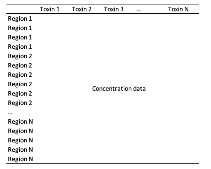
Today, I want to discuss performing column-wise tasks on relatively large datasets. These tasks are particularly common in agricultural and biological research, where we often evaluate multiple experimental subjects across different treatment groups and record a large number of traits for each subject. Under these conditions, the very first step of data analysis is calculating descriptive statistics for every variable across each group of subjects.

What is the best way to do this in R? Let’s explore a few different approaches, starting with a real-life example.

Motivating example

A few days ago, a colleague from our plant pathology group reached out for help analyzing data from a mycotoxin experiment. He studied the concentration of 62 different mycotoxins in wheat caryopses across 70 samples collected from 13 regions in Italy.

The dataset was structured as a 70 x 64 table: one row per wheat sample, the first column containing the sample ID, the second column specifying the region of collection, and the remaining 62 columns containing the concentration levels for each toxin (one column per toxin). The structure of the dataframe is shown below:

My colleague wanted to calculate eight summary statistics for each toxin within each region:

number of collected samples
mean concentration value
maximum concentration value
standard error
number of contaminated samples (where the concentration is higher than 0)
percentage of contaminated samples
mean value for contaminated samples
standard error for contaminated samples

Ultimately, he needed 62 individual summary tables (one per toxin) displaying all 13 regions alongside their respective statistics.

In order to practice with the coding in this post, we’ll use a simulated dataset, which is structured exactly like my colleague’s data and that is available in the ‘statforbiology’ package (the accompanying package for this blog):

library(statforbiology)
dataset <- getAgroData("Mycotoxins")
# str(dataset)
# 'data.frame': 70 obs. of  64 variables:
#  $ Sample : int  1 2 3 4 5 6 7 8 9 10 ...
#  $ Region : chr  "Lombardy" "Lombardy" "Lombardy" "Lombardy" ...
#  $ DON    : num  8.62 16.2 18.19 27.08 10.97 ...
#  $ DON3G  : num  21.7 28.4 34.7 26.9 26.4 ...
# ...
# ...
#  $ QLA    : num  37.5 21 20 26.9 17 ...
#  $ CRV    : num  29.4 32 28.4 9.7 22.7 ...
#  $ VERF   : num  22.1 28.7 17.2 34.4 26.7 ...
#  $ FLAG   : num  26.4 20 27.1 25.8 34.7 ...

A ‘for()’ loop

Long-standing users of general-purpose programming languages, such as Quick-BASIC and Visual Basic, who have transitioned to R quite recently, might have the initial instinct of using a for() loop to repeat the task across columns.

Following this route, we can combine the function tapply() (to compute group-wise statistics) with a for() loop to iterate over the dataset’s columns.

returnList <- list()
range_cols <- c(3:ncol(dataset))
for(i in range_cols){
  y <- dataset[, i]
  Count <- tapply(y, dataset$Region, length)
  Mean <- tapply(y, dataset$Region, mean)
  Max <- tapply(y, dataset$Region, max)
  SE <- tapply(y, dataset$Region, sd)/sqrt(Count)
  nPos <- tapply(y != 0, dataset$Region, sum)
  PercPos <- tapply(y != 0, dataset$Region, mean)*100
  muPos <- tapply(ifelse(y > 0, y, NA), dataset$Region, mean, na.rm = T)
  muPos[is.na(muPos)] <- 0
  sdPos <- tapply(ifelse(y > 0, y, NA), dataset$Region, sd, na.rm = T)
  SEpos <- sdPos/sqrt(nPos)
  returnList[[i]] <- data.frame(cbind(Count, Mean, Max, SE, nPos, PercPos, muPos, SEpos))
  names(returnList)[[i]] <- colnames(dataset)[i]
}
print(returnList$CRV, digits = 2)
##                 Count Mean Max   SE nPos PercPos muPos SEpos
## Abruzzo             4   28  30 0.85    4     100    28  0.85
## Apulia              9   25  40 2.67    9     100    25  2.67
## Campania            2   20  21 0.74    2     100    20  0.74
## Emilia Romagna      8   23  33 2.80    8     100    23  2.80
## Latium              7   20  33 2.76    7     100    20  2.76
## Lombardy            4   25  32 5.12    4     100    25  5.12
## Molise              1   18  18   NA    1     100    18    NA
## Sardinia            6   25  38 3.32    6     100    25  3.32
## Sicily              6   21  30 2.94    6     100    21  2.94
## The Marche          5   19  23 1.58    5     100    19  1.58
## Tuscany             5   30  34 1.22    5     100    30  1.22
## Umbria              9   21  32 2.83    9     100    21  2.83
## Veneto              4   23  28 1.99    4     100    23  1.99

This code works perfectly and feels very natural to me. From a teaching perspective, it also has real value: it introduces students to loops, which are foundational building blocks in computer programming.

However, many R practitioners would consider this solution sub-optimal because for() loops in R can be inefficient. Furthermore, re-using and adapting this code for other projects requires tedious editing and is prone to accidental bugs. Let’s see what other tools R offers for this task.

The `apply()` function

A second classic option is using the apply() function instead of an explicit loop. First, we write a custom helper function (funBec in the code below) to compute group-wise statistics for a single column. Then, we use apply() to sweep that function across every variable column in the dataframe:

funBec <- function(y, group){
  Count <- tapply(y, group, length)
  Mean <- tapply(y, group, mean)
  Max <- tapply(y, group, max)
  SE <- tapply(y, group, sd)/sqrt(Count)
  nPos <- tapply(y != 0, group, sum)
  PercPos <- tapply(y != 0, group, mean)*100
  muPos <- tapply(ifelse(y > 0, y, NA),group, mean, na.rm = T)
  muPos[is.na(muPos)] <- 0
  sdPos <- tapply(ifelse(y > 0, y, NA), group, sd, na.rm = T)
  SEpos <- sdPos/sqrt(nPos)
  data.frame(cbind(Count, Mean, Max, SE, nPos, PercPos, muPos, SEpos))
}
range_cols <- c(3:length(dataset[1,]))
returnList2 <- apply(dataset[range_cols], 2,
                     function(col) funBec(col, dataset$Region))
print(returnList2$CRV, digits = 2)
##                 Count Mean Max   SE nPos PercPos muPos SEpos
## Abruzzo             4   28  30 0.85    4     100    28  0.85
## Apulia              9   25  40 2.67    9     100    25  2.67
## Campania            2   20  21 0.74    2     100    20  0.74
## Emilia Romagna      8   23  33 2.80    8     100    23  2.80
## Latium              7   20  33 2.76    7     100    20  2.76
## Lombardy            4   25  32 5.12    4     100    25  5.12
## Molise              1   18  18   NA    1     100    18    NA
## Sardinia            6   25  38 3.32    6     100    25  3.32
## Sicily              6   21  30 2.94    6     100    21  2.94
## The Marche          5   19  23 1.58    5     100    19  1.58
## Tuscany             5   30  34 1.22    5     100    30  1.22
## Umbria              9   21  32 2.83    9     100    21  2.83
## Veneto              4   23  28 1.99    4     100    23  1.99

Under the hood, this approach isn’t dramatically different from a for() loop, but it feels much more “R-like.” The code is cleaner, more expressive, and far easier to reuse across projects. Still, the helper function contains the method tapply() to summarise across groups, which, to me, doesn’t look good.

A ‘Split-Apply-Combine’ strategy

Another alternative is switching from a column-looping strategy to the ‘split-apply-combine’ paradigm. If we “pivot” (or melt) our wide dataset so that variable measurements are stacked vertically into a single column, we can:

Split the dataset into subsets defined by each unique Toxin-Region pair,
Apply our summary function to calculate statistics for each subset, and
Combine all results back into a clean output structure.

In essence, we transform a tricky ‘column-wise’ task into a straightforward ‘row-wise’ operation.

In base R, we can use reshape() to pivot the data into long format, and aggregate() to calculate our summary metrics using a simplified helper function (funBec2()). Notice how much simpler funBec2() is: because it operates on one single group at a time, we no longer need tapply() inside it! Finally, in order to produce a list of tables (as required by my colleague) we can use split() on the unified output table:

funBec2 <- function(y){
  Count <- length(y)
  Mean <- mean(y)
  Max <- max(y)
  SE <- sd(y)/sqrt(length(y))
  nPos <- sum(y != 0)
  PercPos <- mean(y != 0)*100
  muPos <- mean(ifelse(y > 0, y, NA), na.rm = T)
  muPos[is.na(muPos)] <- 0
  sdPos <- sd(ifelse(y > 0, y, NA), na.rm = T)
  SEpos <- sdPos/sqrt(nPos)
  c("Count"=Count, "Mean" = Mean, "Max" = Max, "SE" = SE,
      "nPos" = nPos, "PercPos" = PercPos, "muPos" = muPos, "SEpos" = SEpos)
}

# Create a dataframe
range_cols <- c(3:length(dataset[1,]))
returnList3 <- dataset |>
  reshape(direction = "long",
          varying = colnames(dataset[range_cols]),
          v.names = "Conc",
          times = colnames(dataset[range_cols]),
          timevar = "Toxin",
          ids = dataset$Sample,
          idvar = "Sample") |>
  aggregate(Conc ~ Region + Toxin, funBec2, simplify = T) |>
  split(~ Toxin)
print(returnList3$CRV, digits = 2)
##              Region Toxin Conc.Count Conc.Mean Conc.Max Conc.SE Conc.nPos
## 235         Abruzzo   CRV       4.00     28.28    29.63    0.85      4.00
## 236          Apulia   CRV       9.00     24.73    39.74    2.67      9.00
## 237        Campania   CRV       2.00     19.80    20.53    0.74      2.00
## 238 Emilia Romagna    CRV       8.00     23.29    33.33    2.80      8.00
## 239          Latium   CRV       7.00     20.38    32.82    2.76      7.00
## 240        Lombardy   CRV       4.00     24.88    32.01    5.12      4.00
## 241          Molise   CRV       1.00     18.14    18.14      NA      1.00
## 242        Sardinia   CRV       6.00     25.31    37.97    3.32      6.00
## 243          Sicily   CRV       6.00     20.74    29.78    2.94      6.00
## 244      The Marche   CRV       5.00     18.50    23.45    1.58      5.00
## 245         Tuscany   CRV       5.00     30.35    33.58    1.22      5.00
## 246          Umbria   CRV       9.00     20.58    32.17    2.83      9.00
## 247          Veneto   CRV       4.00     23.41    28.08    1.99      4.00
##     Conc.PercPos Conc.muPos Conc.SEpos
## 235       100.00      28.28       0.85
## 236       100.00      24.73       2.67
## 237       100.00      19.80       0.74
## 238       100.00      23.29       2.80
## 239       100.00      20.38       2.76
## 240       100.00      24.88       5.12
## 241       100.00      18.14         NA
## 242       100.00      25.31       3.32
## 243       100.00      20.74       2.94
## 244       100.00      18.50       1.58
## 245       100.00      30.35       1.22
## 246       100.00      20.58       2.83
## 247       100.00      23.41       1.99

Alternatively, base R provides the by() function, which accomplishes something similar. However, by() outputs a special object of class ‘by’, which can be tricky to convert into a standard list of dataframes.

When every group yields the exact same set of summary statistics (as in our case), we can coerce the by object into a dataframe using do.call(rbind, ...). However, we must reconstruct the Region and Toxin labels from the dimension names of the array, that is the output of ‘by’. Be extra cautious here: the grouping variables must be specified in the exact same order in both by() and expand.grid(), or your data labels will be misaligned!

returnList4 <- dataset |>
  reshape(direction = "long",
          varying = colnames(dataset[range_cols]),
          v.names = "Conc",
          times = colnames(dataset[range_cols]),
          timevar = "Toxin",
          ids = dataset$Sample,
          idvar = "Sample") |>
  by( ~ Region + Toxin,
      FUN = function(el) funBec2(el$Conc), simplify = T)
  
res_df <- do.call(rbind, returnList4)
grid <- expand.grid(
  Region = dimnames(returnList4)[[1]], 
  Toxin  = dimnames(returnList4)[[2]], 
  stringsAsFactors = FALSE
)
returnList4 <- cbind(grid, res_df)
returnList4 <- split(returnList4, returnList4$Toxin)
print(returnList4$CRV, digits = 4)
##              Region Toxin Count  Mean   Max     SE nPos PercPos muPos  SEpos
## 235         Abruzzo   CRV     4 28.28 29.63 0.8493    4     100 28.28 0.8493
## 236          Apulia   CRV     9 24.73 39.74 2.6657    9     100 24.73 2.6657
## 237        Campania   CRV     2 19.80 20.53 0.7350    2     100 19.80 0.7350
## 238 Emilia Romagna    CRV     8 23.29 33.33 2.7961    8     100 23.29 2.7961
## 239          Latium   CRV     7 20.38 32.82 2.7589    7     100 20.38 2.7589
## 240        Lombardy   CRV     4 24.88 32.01 5.1183    4     100 24.88 5.1183
## 241          Molise   CRV     1 18.14 18.14     NA    1     100 18.14     NA
## 242        Sardinia   CRV     6 25.31 37.97 3.3187    6     100 25.31 3.3187
## 243          Sicily   CRV     6 20.74 29.78 2.9358    6     100 20.74 2.9358
## 244      The Marche   CRV     5 18.50 23.45 1.5836    5     100 18.50 1.5836
## 245         Tuscany   CRV     5 30.35 33.58 1.2218    5     100 30.35 1.2218
## 246          Umbria   CRV     9 20.58 32.17 2.8304    9     100 20.58 2.8304
## 247          Veneto   CRV     4 23.41 28.08 1.9934    4     100 23.41 1.9934

I think that the above coding is less clear than the previous one, where I used the aggregate() function, also because I could not maintain a unique pipeline (in this respect, further pipe optimisation is possible, but the coding becomes harder to read)

The ‘tidyverse approach’

Another solution comes from the tidyverse. Here, we use pivot_longer() to reshape the data, group_by() to establish internal grouping by Region and Toxin and summarise() to calculate all required statistics in one readable block. When passing funBec2(), we must comply with the expectation of summarise() that arguments evaluate to scalar values. Wrapping our function in as_tibble_row() neatly converts the 8-element vector into a single 1-row data frame that summarise() can unpack across columns. The final output is a tidy tibble, which we can split into an unnamed list of tibbles using group_split(). In order to name each element in the list, we use the function setNames() and ‘group_keys()’ to recover the names of toxins (I have to thank my collegue Renzo Bonifazi for suggestions on how to improve the coding below). If we do not want to stick to the tidyverse by all means, we can replace the final line with the function split() from base R, which improves the clarity of coding.

library(tidyverse)
range_cols <- c(3:length(dataset[1,]))
returnList5 <- dataset |>
  select(-Sample) |> 
  pivot_longer(names_to = "Toxin", values_to = "Conc",
               cols = range_cols - 1) |>
  group_by(Toxin, Region) |>
  summarise(as_tibble_row(funBec2(Conc)), 
            .groups = "drop_last") |>
  (function(df) setNames(group_split(df, .keep = FALSE), group_keys(df)$Toxin))()
  # Alternative for the final line in base R
  # split(~Toxin)
print(returnList5$CRV, digits = 2)
## # A tibble: 13 × 9
##    Region            Count  Mean   Max     SE  nPos PercPos muPos  SEpos
##    <chr>             <dbl> <dbl> <dbl>  <dbl> <dbl>   <dbl> <dbl>  <dbl>
##  1 "Abruzzo"             4  28.3  29.6  0.849     4     100  28.3  0.849
##  2 "Apulia"              9  24.7  39.7  2.67      9     100  24.7  2.67 
##  3 "Campania"            2  19.8  20.5  0.735     2     100  19.8  0.735
##  4 "Emilia Romagna "     8  23.3  33.3  2.80      8     100  23.3  2.80 
##  5 "Latium"              7  20.4  32.8  2.76      7     100  20.4  2.76 
##  6 "Lombardy"            4  24.9  32.0  5.12      4     100  24.9  5.12 
##  7 "Molise"              1  18.1  18.1 NA         1     100  18.1 NA    
##  8 "Sardinia"            6  25.3  38.0  3.32      6     100  25.3  3.32 
##  9 "Sicily"              6  20.7  29.8  2.94      6     100  20.7  2.94 
## 10 "The Marche"          5  18.5  23.4  1.58      5     100  18.5  1.58 
## 11 "Tuscany"             5  30.3  33.6  1.22      5     100  30.3  1.22 
## 12 "Umbria"              9  20.6  32.2  2.83      9     100  20.6  2.83 
## 13 "Veneto"              4  23.4  28.1  1.99      4     100  23.4  1.99

Some suggestions from the readers

After sharing an earlier draft of this problem, Bryan Hutchinson (UK) wrote to me to share an elegant solution using ‘data.table’ and ‘DescTools’. If you work with large datasets, the ‘data.table’ package offers incredible speed and concise syntax:

library(data.table)
library(DescTools)
 
dataset <- fread("https://casaonofri.it/_datasets/Mycotoxins.csv", header = T)
tnames <- names(dataset[,-c(1:2)])
 
sum_stats <- function(var) {
  # convert integer to double
  var <- as.numeric(var)
  list(
    mean = mean(var, na.rm = TRUE),
    max = max(var, na.rm = TRUE),
    se = sd(var, na.rm = TRUE) / sqrt(length(var)),
    nPos = length(var >0),
    percPos = length(var >0)/length(var)*100,
    muPos =  mean(var > 0),
    SEpos =  sd(var > 0)/sqrt(length(var > 0))
  )
}
 
df_long <- melt(dataset,
                measure.vars = list(tnames),
                variable.name = "Toxin",
                value.name = "Conc")
 
# df_long[, sum_stats(Conc), .(Toxin, Region)]
df_long[Toxin == "CRV", sum_stats(Conc), .(Toxin, Region)]
## Empty data.table (0 rows and 9 cols): Toxin,Region,mean,max,se,nPos...
# df_long[Region == "Lombardy", sum_stats(Conc), .(Region, Toxin)]

Do you have a different strategy or favorite trick for column-wise operations in R? Drop me an email—I’d love to hear your thoughts and share them here!

Thanks for reading, and happy coding! Don’t forget to check out my new book!

Prof. Andrea Onofri
Department of Agricultural, Food and Environmental Sciences
University of Perugia (Italy)
Send comments to: andrea.onofri@unipg.it

This post was originally published on 2020-12-11