Chapter 12 Simple linear regression
Regression analysis is the hydrogen bomb of the statistics arsenal (C. Wheelan)
In the previous chapters we have presented several ANOVA models to describe the results of experiments characterised by one or more explanatory factors, in the form of nominal variables. We gave ample space to these models because they are widely used in agriculture research and plant breeding, where the aim is, most often, to compare genotypes. However, experiments are often planned to study the effect of quantitative variables, such as a sequence of doses, time elapsed from an event, the density of seeds and so on. In these cases, factor levels represent quantities and the interest is to describe the whole range of responses, beyond the levels that were actually included in the experimental design.
In those conditions, ANOVA models do not fully respect the dataset characteristics, as they concentrate exclusively on the responses to the selected levels for the factors under investigation. Therefore, we need another class of models, usually known as regression models, which we will introduce in these two final chapters.
12.1 Case-study: N fertilisation in wheat
It may be important to state that this is not a real dataset, but it was generated by using Monte Carlo simulation, at the end of Chapter 4. It refers to an experiment aimed at assessing the effect of nitrogen fertilisation on wheat yield and designed with four N doses and four replicates, according to a completely randomised lay-out. The results are reported in Table 12.1 and they can be loaded into R from the usual repository, as shown in the box below.
filePath <- "https://www.casaonofri.it/_datasets/"
fileName <- "NWheat.csv"
file <- paste(filePath, fileName, sep = "")
dataset <- read.csv(file, header=T)
##
## Attaching package: 'reshape'
## The following object is masked from 'package:dplyr':
##
## rename| Dose | 1 | 2 | 3 | 4 |
|---|---|---|---|---|
| 0 | 21.98 | 25.69 | 27.71 | 19.14 |
| 60 | 35.07 | 35.27 | 32.56 | 32.63 |
| 120 | 41.59 | 40.77 | 41.81 | 40.50 |
| 180 | 50.06 | 52.16 | 54.40 | 51.72 |
12.2 Preliminary analysis
Looking at this dataset, we note that it has a similar structure as the dataset proposed in Chapter 7, relating to the one-way ANOVA model. The only difference is that, in this example, the explanatory variable is quantitative, instead of nominal. However, as the first step, it may be useful to forget this characteristic and regard the doses as if they were nominal classes. Therefore, we start by fitting an ANOVA model to this dataset.
As usual, we inspect the residuals for the basic assumptions for linear models; the graphs at Figure 12.1 do not show any relevant deviation and, therefore, we proceed to variance partitioning.
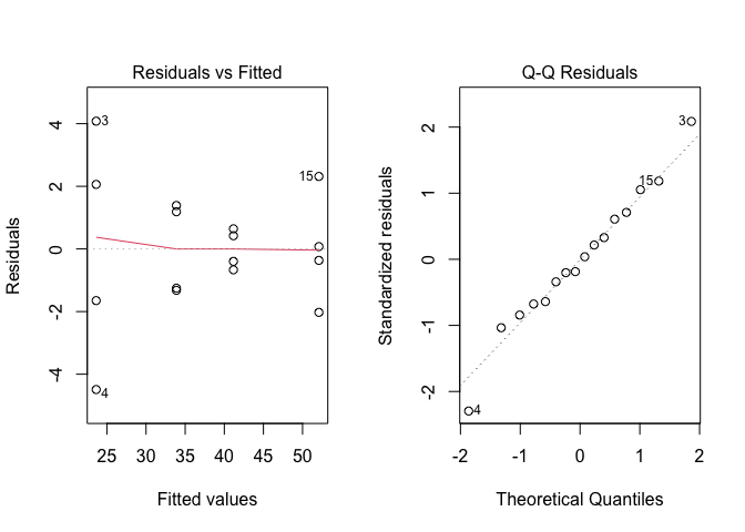
Figure 12.1: Graphical analyses of residuals for a N-fertilisation experiment
anova(modelAov)
## Analysis of Variance Table
##
## Response: Yield
##              Df  Sum Sq Mean Sq F value    Pr(>F)
## factor(Dose)  3 1725.96  575.32  112.77 4.668e-09 ***
## Residuals    12   61.22    5.10
## ---
## Signif. codes:  0 '***' 0.001 '**' 0.01 '*' 0.05 '.' 0.1 ' ' 1
We see that the treatment effect is significant and the residual standard deviation \(\sigma\) is equal to \(\sqrt{5.10} = 2.258\). This is a good estimate of the so-called pure error, measuring the variability between the replicates for each treatment.
In contrast to what we have done in previous chapters, we do not proceed to contrasts and multiple comparison procedures. It would make no sense to compare, e.g., the yield response at 60 kg N ha-1 with that at 120 kg N ha -1; indeed, we are not specifically interested in those two doses, but we are interested in the whole range of responses, from 0 to 180 kg N ha-1. We just selected four rates to cover that interval, but we could have as well selected four different doses, e.g. 0, 55, 125 and 180 kg N ha-1. As we are interested in the whole range of responses, our best option is to fit a regression model, where the dose is regarded as a numeric variabile, which can take all values from 0 to 180 kg N ha-1.
12.3 Definition of a linear model
In this case, we have generated the response by using Monte Carlo simulation and we know that this is linear, within the range from 0 to 180 kg N ha-1. In practice, the regression function is selected according to biological realism and simplicity, keeping into account the shape of the observed response. A linear regression model is:
\[Y_i = b_0 + b_1 X_i + \varepsilon_i\]
where \(Y_i\) is the yield in the \(i\)th plot, treated with a N rate of \(X_i\), \(b_0\) is the intercept (yield level at N = 0) and \(b_1\) is the slope, i.e. the yield increase for 1-unit increase in N dose. The stochastic component \(\varepsilon\) is assumed as homoscedastic and gaussian, with mean equal to 0 and standard deviation equal to \(\sigma\).
12.4 Parameter estimation
In general, we know that parameter estimates for linear models are obtained by using the method of least squares, i.e., by selecting the values that result in the smallest sum of squared residuals. However, for our hand-calculations with ANOVA models, we could use the method of moments, which is very simple and based on means and differences among means. Unfortunately, such a simple method cannot be used for regression models and we have to resort to the general least squares method.
Intuitively, applying this method is rather easy: we need to select the straight line that is the closest to the observed responses. In order to find a algebraic solution, we write the least squares function LS and make some slight mathematical manipulation:
\[\begin{array}{l} LS = \sum\limits_{i = }^N {\left( {{Y_i} - \hat Y_i} \right)^2 = \sum\limits_{i = }^N {{{\left( {{Y_i} - {b_0} - {b_1}{X_i}} \right)}^2}} = } \\ = \sum\limits_{i = }^N {\left( {Y_i^2 + b_0^2 + b_1^2X_i^2 - 2{Y_i}{b_0} - 2{Y_i}{b_1}{X_i} + 2{b_0}{b_1}{X_i}} \right)} = \\ = \sum\limits_{i = }^N {Y_i^2 + Nb_0^2 + b_1^2\sum\limits_{i = }^N {X_i^2 - 2{b_0}\sum\limits_{i = }^N {Y_i^2 - 2{b_1}\sum\limits_{i = }^N {{X_i}{Y_i} + } } } } 2{b_0}{b_1}\sum\limits_{i = }^N {{X_i}} \end{array} \]
where \(\hat{Y_i}\) is the expected value (i.e. \(\hat{Y_i} = b_0 + b_1 X\)). Now, we have to find the values of \(b_0\) and \(b_1\) that result in the minimum value of LS. You may remember from high school that a minimisation problem can be solved by setting the first derivative to zero. In this case, we have two unknown quantities \(b_0\) and \(b_1\), thus we have two partial derivatives, which we can set to zero. By doing so, we get to the following estimating functions:
\[{b_1} = \frac{{\sum\limits_{i = 1}^N {\left[ {\left( {{X_i} - {\mu _X}} \right)\left( {{Y_i} - {\mu _Y}} \right)} \right]} }}{{\sum\limits_{i = 1}^N {{{\left( {{X_i} - {\mu _X}} \right)}^2}} }}\]
and:
\[{b_0} = {\mu _Y} - {b_1}{\mu _X}\]
The hand-calculations, with R, lead to:
X <- dataset$Dose
Y <- dataset$Yield
muX <- mean(X)
muY <- mean(Y)
b1 <- sum((X - muX)*(Y - muY))/sum((X - muX)^2)
b0 <- muY - b1*muX
b0; b1
## [1] 23.79375
## [1] 0.1544167
Hand-calculations look rather outdated, today: we would better fit the model by using the usual lm() function and the summary() method. Please, note that we use the ‘Dose’ vector as such, without transforming it into a factor:
modelReg <- lm(Yield ~ Dose, data = dataset)
summary(modelReg)
##
## Call:
## lm(formula = Yield ~ Dose, data = dataset)
##
## Residuals:
##     Min      1Q  Median      3Q     Max
## -4.6537 -1.5350 -0.4637  1.9250  3.9163
##
## Coefficients:
##              Estimate Std. Error t value Pr(>|t|)
## (Intercept) 23.793750   0.937906   25.37 4.19e-13 ***
## Dose         0.154417   0.008356   18.48 3.13e-11 ***
## ---
## Signif. codes:  0 '***' 0.001 '**' 0.01 '*' 0.05 '.' 0.1 ' ' 1
##
## Residual standard error: 2.242 on 14 degrees of freedom
## Multiple R-squared:  0.9606, Adjusted R-squared:  0.9578
## F-statistic: 341.5 on 1 and 14 DF,  p-value: 3.129e-11
Now, we know that, on average, we can expect that the relationship between wheat yield and N fertilisation dose can be described by using the following model:
\[\hat{Y_i} = 23.794 + 0.154 \times X_i\]
However, we also know that the observed response will not follow the above function, because of the stochastic element \(\varepsilon_i\), which is regarded as gaussian and homoscedastic, with mean equal 0 and standard deviation equal to 2.242 (see the residual standard error in the output above).
Are we sure that the above model provides a good description of our dataset? Let’s investigate this issue.
12.5 Goodness of fit
Regression models need to be inspected with some further attention with respect to ANOVA models. Indeed, we do not only need to verify that the residuals are gaussian and homoscedastic, we also need to carefully verify that model predictions closely follow the observed data (goodness of fit).
The inspection of residuals can be done using the same graphical techniques, as shown for ANOVA models (plot of residuals against expected values and QQ-plot of standardised residuals). In this case, we have already made such inspections with the corresponding ANOVA model and we do not need to do them again with this regression model. However, we need to prove that the linear model provides a good fit to the observed data, which we can accomplish by using several methods.
12.5.1 Graphical evaluation
The first and easiest method to check the goodness of fit is to plot the data along with model predictions, as shown in Figure 12.2. Do we see any deviations from linearity? Clearly, the fitted model provides a good description of the observed data.
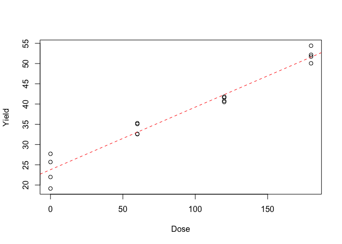
Figure 12.2: Response of wheat yield to N fertilisation: the symbols show the observed data, the dashed line shows the fitted model
12.5.2 Standard errors for parameter estimates
In some cases, looking at the standard error for the estimated parameters may help evaluate whether the fitted model is reasonable. For example, in this case, we might ask ourselves whether the regression line is horizontal, which would mean that wheat yield is not related to N fertilisation. A horizontal line has slope equal to 0, while \(b_1\) was 0.154; however, we also know that \(b_1\) is our best guess for the population slope \(\beta_1\) (do not forget that we have observed a sample, but we are interested in the population). Is it possible that the population slope \(\beta_1\) is, indeed, zero?
If we remember the content of Chapter 5, we can build confidence intervals around an estimate by taking (approximately) twice the standard error. Consequently, the approximate confidence interval for the slope is 0.137705 - 0.171129 and we see that such an interval does not contain 0, which is, therefore, a very unlikely value. This supports the idea that the observed response is, indeed, a linear function of the predictor and that there is no relevant lack of fit.
More formally, we can test the hypothesis \(H_0: \beta_1 = 0\) based on the usual T ratio between an estimate and its standard error:
\[T = \frac{b_1}{SE(b_1)} = \frac{0.154417}{0.008356} = 18.48\]
If the null is true, the sampling distribution for T is a Student’s t, with 14 degrees of freedom. Thus we see that we have obtained a very unlikely T value and the P-value is:
Therefore, we can reject the null and conclude that \(\beta_1 \ne 0\). The t-test for model parameters is reported in the output of the summary() method (see above).
12.5.3 F test for lack of fit
Another formal test is based on comparing the fit of the ANOVA model above (where the dose was regarded as a nominal factor) and the regression model. The residual sum of squares for the ANOVA model is 61.22, while that for the regression model is 70.37 (see the box below).
anova(modelReg)
## Analysis of Variance Table
##
## Response: Yield
##           Df  Sum Sq Mean Sq F value    Pr(>F)
## Dose       1 1716.80 1716.80  341.54 3.129e-11 ***
## Residuals 14   70.37    5.03
## ---
## Signif. codes:  0 '***' 0.001 '**' 0.01 '*' 0.05 '.' 0.1 ' ' 1
Indeed, the ANOVA model appears to provide a better description of the experimental data, which is expected, as the residuals contain only the so-called pure error, i.e. the variability of each value around the group mean. On the other hand, the residuals from the regression model contain an additional component, represented by the distances from group means to the regression line. Such a component is the so-called lack of fit (LF) and it may be estimated as the following difference:
\[\textrm{LF} = 70.37 - 61.22 = 9.15\]
It is perfectly logic to ask ourselves whether the lack of fit component is bigger than the pure error component. We know that we can compare variances based on an F ratio; in this case the number of degrees of freedom for the residuals is 14 for the regression model (16 values minus 2 estimated parameters) and 12 for the ANOVA model (3 \(\times\) 4). Consequently, the lack of fit component has 2 degrees of freedom (14 - 12 = 2). The F ratio for lack of fit is:
\[F_{LF} = \frac{ \frac{RSS_r - RSS_a}{DF_r - DF_a} } {\frac{RSS_a}{DF_a}} = \frac{9.15 / 2}{61.22/12} = 0.896\]
where RSSr is the residual sum of squares for regression, with DFr degrees of freedom and RSSa is the residual sum of squares for ANOVA, with DFa degrees of freedom. More quickly, with R we can use the anova() method, passing both models as arguments:
anova(modelReg, modelAov)
## Analysis of Variance Table
##
## Model 1: Yield ~ Dose
## Model 2: Yield ~ factor(Dose)
##   Res.Df    RSS Df Sum of Sq      F Pr(>F)
## 1     14 70.373
## 2     12 61.219  2    9.1542 0.8972 0.4334
This test is not significant (P > 0.05) and, therefore, we should not reject the null hypothesis of no significant lack of fit effect. Thus, we conclude that the regression model provides a good description of the dataset and it fits as well as an ANOVA model, but it is more parsimonious (in other words, it has a lower number of estimated parameters).
12.5.4 F test for goodness of fit and coefficient of determination
As every other linear models, regression models can be reduced to the model of the mean (null model: \(Y_i = \mu + \varepsilon_i\)) by removing parameters. For example, if we remove \(b_1\), the simple linear regression model reduces to the model of the mean. If you remember from Chapter 4, the model of the mean has no predictors and, therefore, it must be the worst fitting model, as it assumes that we have no explanation for the data.
Hence, we can compare the regression model with the null model and test whether the former is significantly better than the latter. The residual sum of squares for the null model is given in the following box, while we have seen that the residual sum of squares for the regression model is 70.37.
The difference between the null model and the regression model represents the so-called goodness of fit (GF) and it is:
\[GF = 1787.18 - 70.37 = 1716.81\]
The GF value is a measure of how much the fit improves when we add the predictor to the model; we can compare GF with the residual sum of squares from regression, by using another F ratio. The degrees of freedom are, respectively, 1 and 14 for the two sum of squares and, consequently, the F ratio is:
\[ F_{GF} = \frac{\frac{RSS_t - RSS_r}{DF_t - DF_r} } {\frac{RSS_r}{DF_r}} = \frac{1716.81/1}{70.37/14}\]
where RSSt is the residual sum of squares for the null model, with DFt degrees of freedom. In R, we can use the anova() method and we do not even need to include the null model as the argument, as this is included by default:
anova(modelReg)
## Analysis of Variance Table
##
## Response: Yield
##           Df  Sum Sq Mean Sq F value    Pr(>F)
## Dose       1 1716.80 1716.80  341.54 3.129e-11 ***
## Residuals 14   70.37    5.03
## ---
## Signif. codes:  0 '***' 0.001 '**' 0.01 '*' 0.05 '.' 0.1 ' ' 1
The null hypothesis (the goodness of fit is not significant) is rejected and we confirm that the regression model is a good model.
In order to express the goodness of fit, a frequently used statistic is the determination coefficient or R2, i.e. the ratio of the residual sum of squares from regression to the residual sum of squares from the null model:
\[R^2 = \frac{SS_{reg}}{SS_{tot}} = \frac{1716.81}{1787.18} = 0.961\]
This ratio goes from 0 to 1: the highest the value the highest the proportion of the total deviance that can be explained by the regression model (please, remember that the residual sum of squares from the model of the mean corresponds to the total deviance). The determination coefficient is included in the output of the summary() method applied to the ‘modelReg’ object.
12.6 Making predictions
Once we are sure that the model provides a good description of the dataset, we can use it to make predictions for whatever N dose we have in mind, as long as it is included within the minimum and maximum N dose in the experimental design (extrapolations are not allowed). For predictions, we can use the predict() method; it needs two arguments: the model object and the X values to use for the prediction, as a dataframe. In the box below we predict the yield for 30 and 80 kg N ha-1:
pred <- predict(modelReg, newdata=data.frame(Dose=c(30, 80)), se=T)
pred
## $fit
##        1        2
## 28.42625 36.14708
##
## $se.fit
##         1         2
## 0.7519981 0.5666999
##
## $df
## [1] 14
##
## $residual.scale
## [1] 2.242025
It is also useful to make inverse prediction, i.e. to calculate the dose giving a certain response level. For example, we may wonder what N dose we need to obtain a yield of 4.5 q ha-1. To determine this, we need to solve the model for the dose and make the necessary calculations:
\[X = \frac{Y - b_0}{b_1} = \frac{45 - 23.79}{0.154} = 137.33\]
In R, we can use the deltaMethod() function in the car package, that also provides standard errors based on the law of propagation of errors (we spoke about this in a previous chapter):
car::deltaMethod(modelReg, "(45 - b0)/b1",
                 parameterNames=c("b0", "b1"))
##              Estimate       SE    2.5 % 97.5 %
## (45 - b0)/b1 137.3314   4.4424 128.6244 146.04
The above inverse predictions are often used in chemical laboratories for the process of calibration.
12.7 Further readings
- Draper, N.R., Smith, H., 1981. Applied Regression Analysis, in: Applied Regression. John Wiley & Sons, Inc., IDA, pp. 224–241.
- Faraway, J.J., 2002. Practical regression and Anova using R. http://cran.r-project.org/doc/contrib/Faraway-PRA.pdf, R.