Chapter 1 Science and pseudoscience

A witty saying proves nothing (Voltaire)

In the age of ‘information overload’, we have plenty of knowledge at our fingertips. We can ‘google’ for a topic and our computer screen is filled with thousands of links, where we can find every piece of information we are looking for. However, one important question remains unanswered: which information is reliable and scientifically sound? We know by experience that the web is full of personal views, opinions, beliefs or, even worse, fake-news; we have nothing against opinions (although we would rather stay away from fake-news), but we need to be able to distinguish between subjective opinions and objective facts. Let’s refer to the body of reliable and objective knowledge by using the term ‘science’, while all the rest is ‘non-science’ or ‘pseudoscience’; the question is: “How can we draw the line between science and pseudoscience?”. It is a relevant question in these days, isn’t it?

A theory, in itself, is not necessarily science. It may be well-substantiated, it can incorporate good laws and/or equations, it may come either from a brilliant intuition or from a meticulous research work; it may come from a common man or from a very authoritative scientist… it does not matter: theories do not necessarily represent objective facts.

1.1 Science needs data

Theories need to proved. This fundamental innovation is usually attributed to Galileo Galilei (1564-1642), who is usually regarded as the founder of the scientific method, as summarised in Figure 1.1.

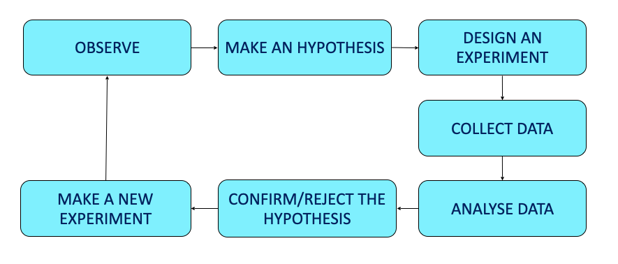
Figure 1.1: The steps to scientific method

Two aspects need attention:

1. the fundamental role of scientific experiments, that produce data in support of pre-existing hypotheses (theories);
2. once a theory has been supported by the data, it is regarded as acceptable until new data disproves it and/or supports an alternative, more reliable or simpler, theory.

Indeed, data is the most important ingredient of science; a very famous aphorism says “In God we trust, all the others bring data”. It is usually attributed to the American statistician, engineer and professor W. Edwards Deming (1900-1993), although it is also attributed to Robert W. Hayden. Trevor Hastie, Robert Tibshirani and Jerome Friedman, the authors of the famous book ‘The Elements of Statistical Learning’, mention that Professor Hayden told them that he cannot claim any credit for the above quote. A search on the web shows that there is no data confirming that W.E. Deming is the author of the above aphorism. Rather funny; I have just reported a sentence stating the importance of data in science, although it would appear that my attribution is just an unsupported theory!

1.2 Not all data support science

Science is based on data, but we need to be careful: not all data can be trusted. In agriculture and, more generally, in biology and other quantitative sciences, we usually deal with measurable phenomena and, therefore, our data consists of a set of measurements of several types (we’ll come back to this in Chapter 2).

For a number of reasons, each measure may not exactly reflect the true value and such a difference is usually known as experimental error. This final word (‘error’) should not mislead you: it does not necessarily mean that we are doing something wrong. On the contrary, errors are regarded as an unavoidable component of all experiments, injecting uncertainty in all the observed results.

We can list three fundamental sources of uncertainty:

1. measurement error
2. subject-to-subject variability
3. sampling error

Measurement errors can be due, e.g., to: (i) uncalibrated instruments, (ii) incorrect measurement protocols, (iii) failures of the measuring devices, (iv) reading/writing errors and other inaccuracies relating to the experimenter’s work and (v) irregularities in the object being measured. In this latter respect, taking, e.g., the precise diameter of a melon is very difficult, as this fruit is not characterised by a regular spherical shape and, furthermore, the observed value is highly dependent on the point where the measurement is taken.

Apart from measurement errors, there are other, less obvious, sources of uncertainty. In particular, we should keep into account that research studies in agriculture and biology need to consider a population of individuals; for instance, think that we have to measure the effect of a herbicide on a certain weed species, by assessing the weight reduction of treated plants. Clearly, we cannot just measure one plant, but we have to make a number of measurements on a population of weed plants. Even if we managed to avoid all measurement errors (which is nearly impossible), the observed values would always be different from one another, due to a more or less high degree of subject-to-subject variability. Such an uncertainty does not relate to any type of technical error, but it is an inherent component of the biological process under investigation.

Subject-to-subject variability would not be, in itself, a big problem, if we could measure all individuals; unfortunately, populations are so big that we are obliged to measure a small sample and we can never be sure that the observed value for the sample matches the real value for the whole population. Of course, we should do our best to select a representative sample, but we already know that the ‘perfect sample’ does not exist and, in the end, we are always left with several dobts. Was our sample representative? Did we left out some important group of individuals? What will it happen, if we take another sample?

In other words, uncertainty is an intrinsic and unavoidable component of all data and, therefore, how can we decide when the data are good enough to support science?

1.3 Good data is based on good ‘methods’

Uncertainty is produced by errors (sensu lato as we said above), but not all errors are created equal! In particular we need to distinguish systematic errors from random errors. Systematic errors tend to occur repeatedly with the same sign; for example, think about an uncalibrated scale, producing always a 20% weight overestimation: we can do as many measurements as we want, but the experimental error will be most often positive. Or, think about a technician, who is following a wrong measuring protocol.

On the other hand, random errors relate to unknown, unpredictable and episodic events, producing repeated measures that are different from each other and from the true value. Due to such random nature, random errors have random signs; they may be positive or negative and, at least on the long run, they are expected to produce underestimations or overestimations with equal probability.

It is easy to grasp that the consequences of those two types of errors are totally different. In this respect, it will be useful to consider two important traits of a certain body of data:

1. precision
2. accuracy

The term precision is usually seen as the ability of discriminating small differences; in this sense, a standard ruler can measure lengths to the nearest millimetre and it is less precise than a calliper, that can measure lengths to the nearest 0.01 millimetre. However, in biometry, the term precision is more often used to mean low variability of results when measurements are repeated. The term accuracy has a totally different meaning and it refers to any possible differences between a measure and the corresponding ‘true’ value. The typical example is an uncalibrated instrument: the measures in themselves can be very precise, but they are inaccurate, because they do not correspond to the real value.

We clearly understand that precision is important, but accuracy is fundamental; inaccurate data are said to be biased. Random errors result in imprecise data, but they do not necessary lead to biased data, as we can assume that repeating the measures for a reasonable amount of times should bring to a reliable estimate of the true unknown value (we will be back to this issue later). On the contrary, systematic errors lead to inaccurate (biased) data and wrong conclusions; therefore, they need to be avoided by any possible means, which must be the central objective of all experimental studies. In this sense, perfect instrument calibration and rigorous measurement and sampling protocols play a fundamental role, as we will see later.

Unfortunately, inaccurate data and wrong conclusions are not uncommon in science; one of the most famous case was when the American scientists Martin Fleischmann and Stanley Pons, on 23 March 1989, published the results of an important experiment, claiming that they had produced a nuclear reaction at room temperature (cold fusion). Fleischmann and Pons’ announcement drew wide media attention (see Figure 1.2), but several scientists failed to reproduce the results in independent experiments. Later on, several flaws and sources of experimental error were discovered in the original experiment and most scientists considered cold fusion claims dead. Subsequently, cold fusion gained a reputation as pathological science and was marginalised by the wider scientific community, even though a minority of scientists is still investigating on that.

Figure 1.2: Consequences of a wrong experiment, producing bad data.

Apart from that famous example, we need to go back to our original question: how can we be sure that the data are accurate? The answer is simple: we can never be totally sure, but we should strive to apply research methods as rigorous as possible, so that we can be as sure as possible that the experiment is ‘valid’, i.e. that it does not contain any sources of systematic error (bias). In other words, good data come as the consequence of valid methods, which implies that a scientific proof is such not because we are certain that it corresponds to the truth, but because we are reasonably certain that it was obtained by using valid methods!

1.4 The ‘falsification’ principle

The above approach has an important consequence: even if we have used a perfectly valid method and we have, therefore, produced a perfectly valid scientific proof, we can never be sure that we are right, because there could always be a future observation that says we are wrong. This is the basis of the ‘falsification theory’, as defined by Karl Popper (1902 – 1994): we cannot demonstrate that our data are true, but we can only demonstrate that they are false.

In practice, going back to the scientific process, we start from our hypothesis, we design a valid experiment and obtain valid data. In case this data does not appear to contradict the hypothesis, we conclude that such a hypothesis is true because it has not been falsified. The hypothesis is held as true until new valid data arise that falsify it: in this instance, the hypothesis is rejected and a new one is defined and submitted to the falsification process.

The falsification theory has been very influential in science. I would like to highlight a few key-points.

1. Science has nothing to do with truth or certainty. Science has a lot to do with uncertainty and we can never prove that a hypothesis is totally right. Therefore, we always organise experiments to reject hypothesis (i.e. to prove that they are false)!
2. We need to use valid methods to ensure that random errors have been minimised, while systematic errors have been avoided as much as possible.
3. The remaining uncertainty due to residual random errors need to be quantified by using the appropriate stats and displayed along with the results.
4. Considering the residual uncertainty, we need to evaluate whether our data are good enough to falsify the original hypothesis. Otherwise, the experiment is inconclusive (but not necessarily the original hypothesis is true!)
5. If we have two competing hypothesis and they are equally good, we select the simplest one (Occam’s razor principle)

1.5 Trying to falsify a result

One aspect to be highlighted is that if I want to try and falsify a hypothesis which has been validated by a previous experiment, I need to organise a confirmatory experiment. In this frame, we need to distinguish between:

1. replicability
2. reproducibility

An experiment is replicable when it gives the same results when repeated in the very same conditions. This explains why an accurate descriptions of materials and methods is fundamental to every scientific report: how could we repeat an experiment without knowing all detail about it?

Unfortunately, field experiments in agriculture are very seldom replicable, due to the environmental conditions, which change unpredictably from one season to the other. Therefore, we can only try to demonstrate that an experiment is reproducible, that is to say that it gives similar results when it is repeated in different conditions. Of course, failing to reproduce the results of an experiment in different conditions does not necessarily negate the validity of the original results.

This latter aspect is relevant. Think about Newton’s gravitation law, which has always worked very well to predict the motion of planets as well as objects on Earth. This law was falsified by Einstein’s studies, but it was not totally abandoned; indeed, within the limits of the conditions where it was proved, Newton’s laws are still valid and they are good enough to be used for relevant tasks, such as to plan the trajectory of rockets.

---

1.6 The basic principles of experimental design

So far, we have seen that we need good data to express scientific claims and, to have good data, we need a valid experiment. A good methodology for designing experiments has been described by the English scientist Ronald A. Fisher (1890 - 1962). He graduated in 1912 and worked for six years as a statistician for the City of London, until he became a member of the Eugenics Education Society of Cambridge, founded in 1909 by Francis Galton, the cousin of Charles Darwin. After the end of the First World War, in 1919 he was offered a position at the Galton Laboratory at the University College of London, led by Karl Pearson, but he refused, due to profound rivalry with Pearson himself. Therefore, he begun working at the Rothamsted Experimental Station (Harpenden), where he was busy analysing the vast body of data that had accumulated starting from 1842. During this period, he invented the analysis of variance and defined the basis for valid experiments, publishing his results in the famous book “The design of experiments”, dating back to 1935.

In summary, Fisher recognised that a valid experiment must adhere to three fundamental principles:

1. control;
2. replication;
3. randomisation.

1.6.1 Control

The term ‘control’ is very often mentioned in Fisher’s book, with a number of different meanings. Perhaps, the most convincing definition is given at the beginning of Chapter 6: ‘control’ consists of establishing controlled conditions, in which all factors except one can be held constant. We can slightly widen this definition by saying that there should not be any difference between experimental units, apart from those factors which are under investigation.

The above definition sets the basis for what we call a comparative experiment; I will better explain this concept by using an example. Just assume that we have found a revolutionary fertiliser and we want to compare it with a traditional one: clearly, we cannot use the innovative fertiliser in one field and compare the observed yield with that obtained in the previous season with the traditional fertiliser. We all understand that, apart from the fertiliser, several environmental variables changed from one season to the other.

A good controlled experiment would consist of using two field plots next to each other, with the same environmental condition, soil, crop genotype and everything else, apart from the fertiliser, which will be different for the two plots. In these conditions, the observed yield difference shall be reasonably attributed to the fertiliser.

Apart from isolating the effect under study, a good control is exerted by using the greatest care to minimise the effects of all potential sources of experimental error. This may seem obvious, but putting it into practice may be overwhelming. Indeed, different types of experiments will require different types of techniques and the best to do to master those techniques is ‘learning by doing’, preferably under the supervision of an expert technician. I will only underline three general aspects:

1. methodological rigour
2. accurate selection of experimental units
3. avoiding intrusions

Methodological rigor refers to the soundness or precision of a study in terms of planning, data collection, analysis, and reporting. It is obvious that, if we intend to study the degradation of a herbicide at 20°C we need an oven that is able to keep that temperature constant, the herbicide needs to be thoroughly mixed with the soil at the exact concentration and we need to use a well calibrated instrument as well as a correct protocol of analysis. However, we should never forget that there is a trade-off between methodological rigour/precision and the need for time and money resources, which is not independent from the aims of the experiment and the expected effect size. It is not necessary to attain a precision of 1 mL if we are determining the irrigation volume for maize!

In relation to the selection of experimental units, good control practices would suggest that we select very homogeneous individuals; by doing so, error is minimised and precision is maximised. However, we need to be careful: subjects also need to reliably represent the population from where they were selected. For instance, if we want to assess the effect of a particular diet, we could select cows of the same age, same weight and same sex, so that the diet effect is isolated from all other possible confounding effects. If we do so, we will probably obtain a very high precision, but our results will not allow for any sound generalisations to caws of other ages, weights and sex. Again, there is a trade-off between the homogeneity of experimental subjects and the possibility of generalisation.

Last, but not least, I would like to spend a few words about ‘intrusions’, i.e. all the external events that occur and negatively impact on the experiment (e.g., drought, fungi attacks, aphids). Sometimes, these events are simply unpredictable and we will see that replication and randomisation (the other two principles of experimental design) are mainly meant to avoid that such intrusions produce systematic errors in our results. Some other times, these events are not totally unpredictable and they are named ‘demonic intrusions’ by Hurlbert (1984) in a very influential paper (as opposed to the unpredictable non-demonic intrusions). The aforementioned author reports an example relating to a study about fox predation. If fences are used to avoid the entrance of foxes, but hawks use those fences as perches from which to search for a pray, in the end, foxes may be held responsible for the predation exerted by hawks. Therefore, we end up confounding the effect of an intrusion with the effect under investigation. Hurlbert concludes “Whether such non-malevolent entities are regarded as demons or whether one simply attributes the problem to the experimenter’s lack of foresight and the inadequacy of procedural controls is a subjective matter. It will depend on whether we believe that a reasonably thoughtful experimenter should have been able to foresee the intrusion and taken steps to forestall it”.

1.6.2 Replication

In the previous paragraph, we have set the basis of a comparative experiment, wherein two plots put totally in the same conditions are treated with two different fertilisers. Of course, this is not enough to guarantee that the experiment is valid. Indeed, no one would now dream of testing the response to a treatment by comparing two plots, one treated and the other one untreated (Fisher and Wishart, 1930; cited in Hurlbert, 1984).

In every valid experiment, the measurements should be replicated in more than one experimental unit, while non-replicated experiments are usually invalid. We can list four main reasons for replication:

1. demonstrate that the measure is replicable (that does not mean it is reproducible, though);
2. ensure that any possible intrusions that affected one single experimental unit has not caused any relevant bias. Of course, the situation becomes troublesome if such an intrusion has affected all replicates! However, we will show that we can take care of this by using randomisation;
3. assess the precision of the experiment, by measuring the variability among replicates;
4. increase the precision of the experiment: the higher the number of replicates the higher the precision and the lower the uncertainty.

The key issue about replication is that, to be valid, replicates must be truly independent, i.e. the whole manipulation process to allocate the treatment must have been independently applied to the different replicates. This must be clearly distinguished from pseudo-replication, where at least part of the manipulation has been contemporarily applied to all replicates (Figure 1.3).

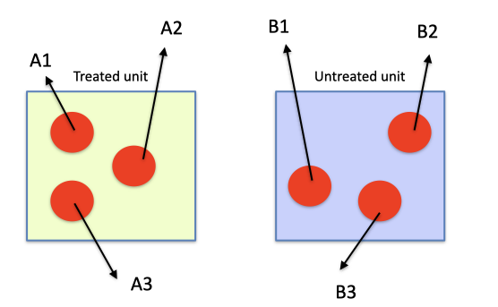
Figure 1.3: Schematic example of and invalid experiment, where pseudo-replication is committed

Some typical examples of pseudo-replication are: (1) spraying a pot with five plants and measuring separately the weight of each plant, (2) treating one soil sample with one herbicide and making four measurements of concentration on four subsamples of the same soil, (3) collecting one soil sample from a field plot and repeating four times the same chemical analysis. In all the above cases, the treatments are applied only to one unit (pot or soil sample) and there are no true replicates, no matter how often the unit is sub-sampled. Clearly, if a random error is committed during the manipulation process, it carries over to all replicates and becomes a very dangerous systematic error.

In some cases, pseudo-replication is less evident and less dangerous; for example, when we have to spray a number of replicates with the same herbicide solution, we should prepare different lots of the same solution and independently spray them onto the replicated plots. In practise, very often we only prepare one solution and spray it onto all the replicates, one after the other. Strictly speaking, this would not be correct, because the manipulation is not totally independent: if we made a mistake while preparing the solution (e.g. a wrong concentration), this would affect all replicates and would become a source of bias. However, such a practice is usually regarded as acceptable: if we sprayed the replicates independently, the amount of solution would too small to be precisely delivered by, e.g., a knapsack sprayer. As always, experience and common sense can be good guides to designing valid experiments.

Apart from some specific circumstances, the general rule is that valid experiments require true-replicates and pseudo-replication should never be mistaken for true replication, even in the case of laboratory experiments (Morrison & Morris, 2000). You will learn by experience the exceptions to this rule, but we prefer to sound rather prescriptive in this respect: it is not nice to have a paper rejected because we did not menage to convince the editor that our lack of true-replication should be regarded as justified!

One common question is: how many replicates do we need? In this respect, we need to find a good balance between precision and costs: four replicates are usually employed in field experiments, although also three is a common value, when the effects are expected to be rather big and we have a small budget. A higher number of replicates is not very common, mainly because the size of the experiment becomes rather big and, consequently, soil variability increases as well.

1.6.3 Randomisation

Control and true-replication, in themselves, do not guarantee that the experiment is valid. Indeed, some innate characteristics of experimental units or some random intrusion might systematically influence all replicates of one treatment, so that the effect of such disturbance is confounded with the effect of the experimental treatment. For example, think that we have a field with eight plots, along a positive gradient of fertility, as shown in Figure 1.4; if we treat the plots from 1 to 4 with the fertiliser A and the plots from 5 to 8 with the fertiliser B, a possible difference between the means for A and B might be wrongly attributed to the treatment effect, while it might be due to the innate difference in fertility (confounding effect).

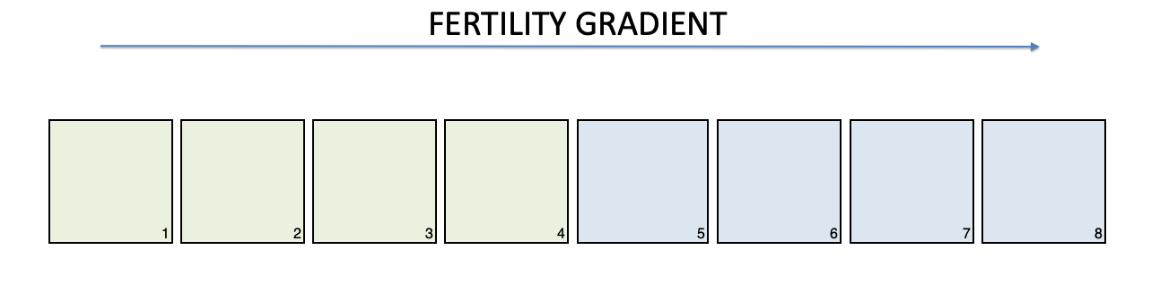
Figure 1.4: Example of lack of randomisation: the colours identify two different experimental treatments

Randomisation is usually performed by way of random allocation of treatments to the experimental units, which is typical of manipulative experiments. In the case of field experiments, randomisation can also relate to random spatial and temporal dispersion, as we will see in the next Chapter.

The allocation of treatments is not always possible, as it may sometimes be impractical, unethical or illegal. For example, if we want to assess the efficacy of seat belts, designing an experiment where people are sent out either with or without fastened seat belts is neither ethical nor legal. In this case, we can only record, retrospectively, the outcome of previous accidents.

In this type of experiment we do not allocate the treatments, but we observe units that are ‘naturally’ treated (observational experiment); therefore, randomisation is obtained by random selection of individuals.

As the result of using proper randomisation, all experimental units are equally likely to receive any type of disturbance/intrusion, so that the probability that all replicates of the same treatment are affected is minimal. Therefore, confounding the effect of a treatment with other types of systematic effects, if not impossible, is made highly unlikely.

1.7 Invalid experiments

Let’s go back to the beginning of this chapter: how do we recognise real science from pseudo-science? By now, we should have learnt that reliable scientific information comes from data obtained in valid experiments. And we should have also learnt that experiments are valid if (and only if) they are properly controlled, replicated and randomised: the lack of any of these fundamental traits makes the results more or less unreliable and doubtful.

In our experience as reviewers and statistical consultants, we have found several instances of invalid experiments. It is a pity: in such cases, the paper is rejected and there is hardly any remedy to a poorly designed experiment. The most frequent problems are:

1. lack of good control
2. ‘Confounding’ and spurious correlation
3. Lack of true replicates and/or careless randomisation

The consequences may be very different.

1.7.1 Lack of good control

In some cases, experiments are not perfectly controlled. Perhaps, this statement is difficult to be interpreted, as no experiments can, indeed, be perfectly controlled: even if we have managed to totally avoid measurement errors, subject-to-subject variability and sampling variability can never be erased. Therefore, in terms of control, how do we draw the line between a valid and an invalid experiment? The suggestion is to carefully check whether the control was good enough not to impact on accuracy. If the experiment was only imprecise, the results do not loose their validity, although they may not be strong enough to reject our initial hypothesis. In other words, imprecise experiments are valid, but, very often, inconclusive. We say that they are not powerful.

An experiment becomes invalid when there are reasons to suspect that the lack of good control impacted on data accuracy (wrong sampling, systematic errors, invalid or unacceptable methods). In this case, the experiment should be rejected, because it might be reporting measures that do not correspond to reality.

1.7.2 ‘Confounding’ and spurious correlation

Reporting wrong measures is dangerous but confounding is even worse. It happens when the effect of some experimental treatments is confounded with other random or non-random systematic effects. The risk is particularly high with observational experiments. For example, if we observe the relative risk of death for individuals who were naturally exposed to a certain risk factor compared to individuals who were not exposed, the experimental outcome can be affected by several uncontrollable traits, such as sex, height, weight, age and so on. Therefore, we have a stimulus (exposure factor), a response (risk of death) and other external variables, which we call the ‘confounders’. If one of the confounders is correlated both with the response and with the stimulus, a ‘spurious’ correlation may appear between the stimulus and the response, which does not reflect any real causal effects (Figure 1.5).

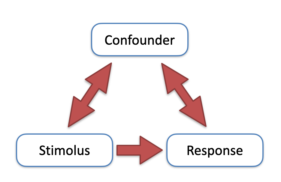
Figure 1.5: Graphical representation of spurious correlation: an external confounder influences both the stimulus and the response, so that these two latter variables are correlated

One typical example of spurious correlation has been found between the number of churches and the number of crimes in American cities. Such a correlation, in itself, does not prove that one factor (religiosity) causes the other one (crime); a thorough explanation should consider the existence of a possible confounder, such as the density of population: big cities have more inhabitants and, consequently, more churches and more crimes with respect to small cities. Accordingly, religiosity and crime are related to density and are related to each other, but such a relationship os only spurious.

In the web, we can found a lot of other funny examples of spurious correlations, such as between the consumption of sour cream over years and the number of motorcycle riders killed in accidents (Figure 1.6). In this case, the lack of any scientific bases is clear; in other cases, it may be more difficult to spot. A very witty saying is: “correlation does not mean causation”; please, do not forget it!

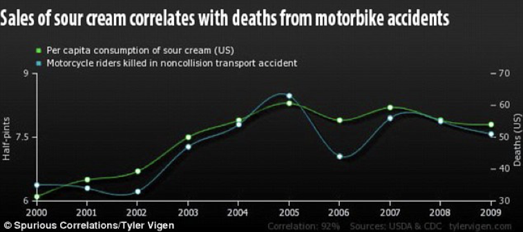
Figure 1.6: Esempio di correlazione spuria

1.7.3 Lack of true-replicates or careless randomisation

Some issues that may lead to the immediate rejection of scientific papers are:

1. there are pseudo-replicates, but no true-replicates
2. true-replicates and pseudo-replicates are mistaken
3. there is no randomisation
4. randomisation was constrained, but the constraint has not been accounted for in statistical analyses.

It is very useful to take a look at the classification made by Hurlbert (1984), which we present in Figure 1.7.

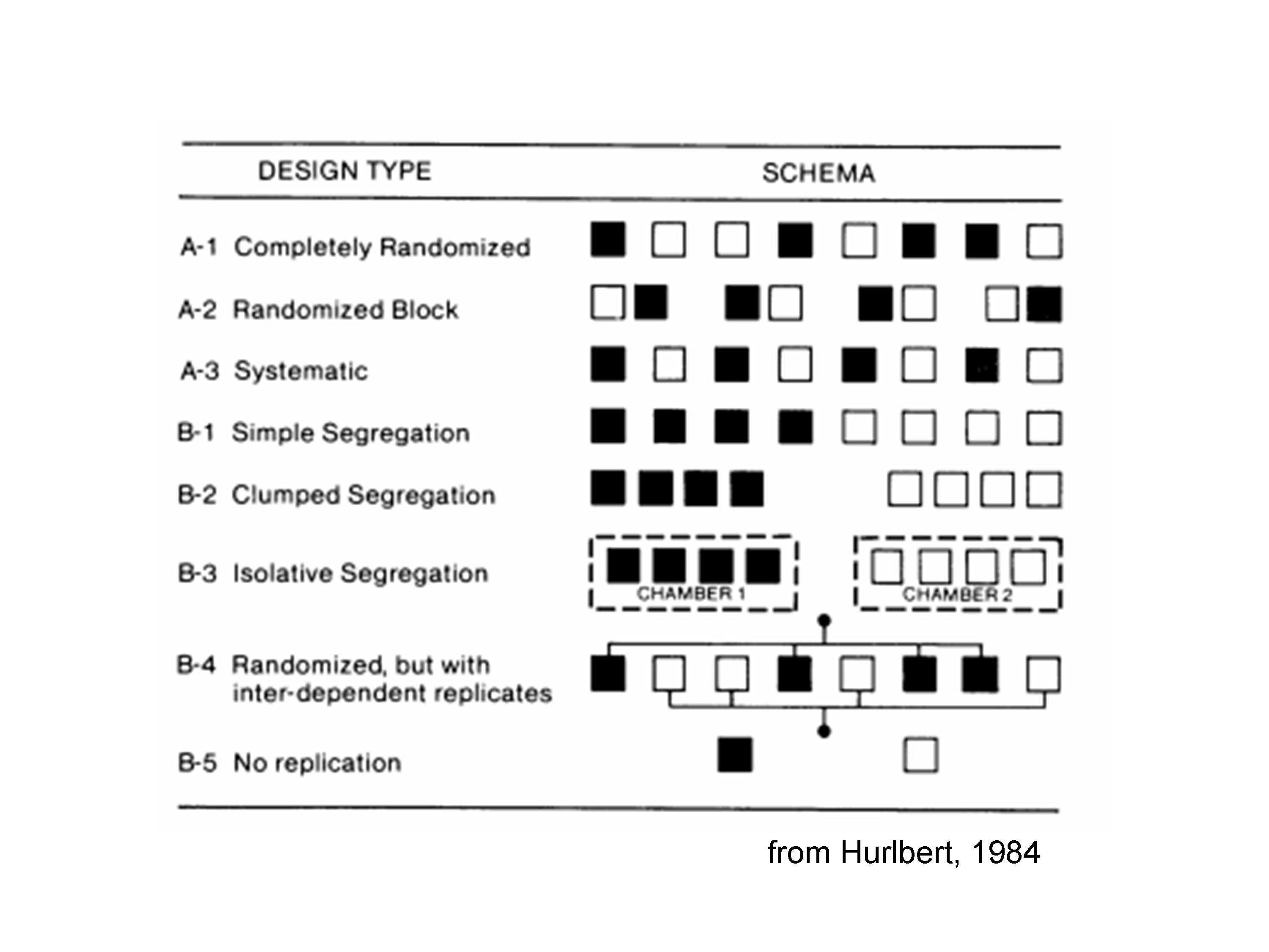
Figure 1.7: Different types of randomisations, although they are not all correct (taken from: Hurlbert, 1984)! See the text for more explanations.

It shows eight experimental subjects, to which two treatments (black and white) were allocated, by using eight different experimental designs. Design A1 is perfectly valid, as the four ‘white’ units and the four ‘black’ units were randomly selected.

Design A2 is correct, although the randomisation was not complete; indeed, we divided the units in four groups and, within each group, we made a random selection of the ‘white’ and ‘black’ individual. This is an example of constrained randomisation, as the random selection of individuals is forced to take place within each group. We will see that such a constraint is correct, but it must be taken into account during the process of data analysis.

Design A3 looks suspicious: there are true replicates, but treatments were not randomly, but systematically allocated to experimental units. Indeed, black units are always to the right of white units; what would happen in case of a latent right-to-left fertility gradient? Black units would be advantaged and the treatment effect and fertility effect would be confounded. Such suspect may lead to an invalid experiment. Systematic allocation of treatments may be permitted in some instances, when a spatial-temporal sequence has to be evaluated. For example:

1. when we have four trees and we want to compare the yield of a low branch with the yield of a high branch. Clearly, low and high branches are systematically ordered and cannot be randomised;
2. when we need to compare herbicide treatments in two timings (e.g., pre-emergence and post-emergence); clearly, one timing is always before the other one;
3. when we need to compare the amount of herbicide residuals at two different depths, which are always ordered along the soil profile.

In those conditions, the experiment is valid even when the randomisation follows a systematic pattern.

Design B1 is usually invalid: there is no randomisation and the systematic allocation of treatments creates the segregation of units, which are not interspersed. The treatment effect can be easily confounded with any possible location effects (right vs. left). Also for design B1, there are a few exceptions were such a design could be regarded as valid, e.g., when we want to compare two locations, two regions, two fields, two lakes or any other physically parted conditions. Such location effects need to be evaluated with great care, as we are rarely in the condition of clearly attributing the effect to a specific agronomic factor. For example, two locations can give different yields because of different soil, different weather, different sowing times and so on.

Design B2 and B3 are analogous to B1, even though the location effects are usually bigger. Isolative segregation is typical of growth chamber experiments; for example, we can use such a design to compare the germination capability at two different temperatures, by using two different ovens. In this case the temperature effect is totally confounded with the oven effect; it may not be problem in case the two ovens are very similar, but it is clear that any malfunctioning of one of the two ovens will be confounded with the treatment effect. Furthermore, the different replicates in one oven are not, indeed, true replicates, because the temperature treatment is not independently allocated (pseudo-replicates).

Design B4 is a general example of pseudo-replication, where replicates are inter-dependent; we have already given other examples in the previous paragraphs. Designs lacking true-replicates are generally invalid, unless true-replicates are also included. For example, if we have four ovens that are randomly allocated to two temperatures (two ovens per temperature) and we have four Petri dishes per oven, there are two true-replicates and four pseudo-replicates per replicate. The design is valid, although we should keep true-replicates and pseudo-replicates clearly parted during data analysis, i.e. we should not behave as if we had 4 \(\times\) 2 = 8 true-replicates!

Design B5 is clearly invalid, due to total lack of replication.

1.8 How can we assess whether the data is valid?

As we said, we have to check the methods. However, in everyday life this is very seldom possible. Indeed, we may not be expert enough to spot possible shortcomings and, above all, the methods may not detailed in newspapers and magazines, which limit themselves to reporting the result. What can we do, then? The answer is simple: we have to carefully check the sources.

Authoritative scientific journals publish manuscripts only after a process of ‘peer review’. In practise, the submitted manuscript is managed by the handling editor, who reads the paper and sends it to one to three widely renowned experts (reviewers). The editor and reviewers carefully inspect the paper and decide whether it can be published either as it is, or after revision, or, on the other hand, it should be rejected. After this process, we can be reasonably sure that the results are reliable and there are no important shortcomings that would make the experiment invalid. The peer review process is rather demanding for authors and it may require months and two-three reviews before the paper is accepted. We have found a nice picture at scienceBlog.com, which summarises rather well the feelings of a scientists during the reviewing process (Figure 1.8).

Figure 1.8: The peer review process

1.9 Conclusions

In the end, we can go back to our initial question: “How can we draw the line between science and pseudoscience?”. The answer is that science is based on reliable data, obtained in valid scientific experiments, wherein every possibile source of systematic errors and confounding has been properly controlled and minimised. In particular, we have seen that every valid experiment should adhere to three fundamental principles, i.e. control, replication and randomisation.

In practice, making sure that the methods were appropriate may require a specific expertise in a certain research field. Therefore, our ‘take-home message’ is: unless we are particularly expert in a given subject, we should always make sure that the results were published in authoritative journals and selected by a thorough peer review process.

---

1.10 Further readings

1. Fisher, Ronald A. (1971) [1935]. The Design of Experiments (9th ed.). Macmillan. ISBN 0-02-844690-9.
2. Hurlbert, S., 1984. Pseudoreplication and the design of ecological experiments. Ecological Monographs, 54, 187-211
3. Kuehl, R. O., 2000. Design of experiments: statistical principles of research design and analysis. Duxbury Press (CHAPTER 1)
4. Morrison, D.A. and Morris, E.C., 2000. Pseudoreplication in experimental designs for the manipulation of seed germination treatments. Austral Ecology 25, 292–296.
5. Wollaston V., 2014. Does sour cream cause bike accidents? No, but it looks like it does: Hilarious graphs reveal how statistics can create false connections. Published at: https://www.dailymail.co.uk/sciencetech/article-2640550/Does-sour-cream-cause-bike-accidents-No-looks-like-does-Graphs-reveal-statistics-produce-false-connections.html. Date of last access: 03/09/2020.