Chapter 12 Plots of different sizes

Factorial experiments are not only laid down with completely randomised designs or in complete blocks. In chapter 2, we have already introduced split-plot or strip-plot designs, where treatment levels are allocated to the experimental units in groups. We have seen that this is advantageous in some circumstances, e.g., when one of the factors is better allocated to bigger plots, compared to the other factors. When factor levels are allocated to groups of individuals, the independency of residuals is broken, as the individuals within the group are more alike than the individuals in different groups. For example, let’s consider a field experiment: if one group of plots is, e.g., more fertile than the other groups, all plots within that group will share such a positive effect and, therefore, their yields will be correlated. In this case, we talk about intra-class correlation, that is a similar concept to the Pearson correlation, which we have encountered in Chapter 3.

In order to respect the basic assumption of independent residuals, data from split-plot and strip-plot experiments cannot be analysed by using the methods proposed in Chapter 11 (multi-way ANOVA models), but they require a different approach.

12.1 Example 1: a split-plot experiment

In chapter 2, we presented an experiment to compare three types of tillage (minimum tillage = MIN; shallow ploughing = SP; deep ploughing = DP) and two types of chemical weed control methods (broadcast = TOT; in-furrow = PART). This experiment was designed in four complete blocks with three main-plots per block, split into two sub-plots per main-plot; the three types of tillage were randomly allocated to the main-plots, while the two weed control treatments were randomly allocated to sub-plots (see Figure 2.9).

The results of this experiment are reported in the ‘beet.csv’ file, that is available in the online repository. In the following box we load the file and transform the explanatory variables into factors.

dataset <- read.csv("https://www.casaonofri.it/_datasets/beet.csv", header=T)
dataset$Tillage <- factor(dataset$Tillage)
dataset$WeedControl <- factor(dataset$WeedControl)
dataset$Block <- factor(dataset$Block)
head(dataset)
##   Tillage WeedControl Block  Yield
## 1     MIN         TOT     1 11.614
## 2     MIN         TOT     2  9.283
## 3     MIN         TOT     3  7.019
## 4     MIN         TOT     4  8.015
## 5     MIN        PART     1  5.117
## 6     MIN        PART     2  4.306

By looking at the map in Figure 2.9, it is easy to see that there are two types of constraints to randomisation:

each replicate of the six combinations was allocated to each block
the two weed control methods were allocated to each main plot

As the consequence, apart from treatment factors, we have two blocking factors, i.e. the blocks and the main-plots within each block; Both this blocking factors should be included in the model, in order to ensure the independence of residuals.

12.1.1 Model definition

Considering the above comments, a linear model for a two-way split-plot experiment is:

\[Y_{ijk} = \mu + \gamma_k + \alpha_i + \theta_{ik} + \beta_j + \alpha\beta_{ij} + \varepsilon_{ijk}\]

where \(\gamma\) is the effect of the \(k\)^th block, \(\alpha\) is the effect of the \(i\)^th tillage, \(\beta\) is the effect of \(j\)^th weed control method, \(\alpha\beta\) is the interaction between the \(i\)^th tillage method and \(j\)^th weed control method. Apart from these effects, which are totally the same as those used in Chapter 11, we also include the main-plot effect \(\theta\), where we use the \(i\) and \(k\) subscripts, as each main-plot is uniquely identified by the block to which it belongs and by the tillage method with which it was treated (see Figure 2.9). Obviously, the main plots can be labelled in any other way, as long as each one is uniquely identified.

Now, let’s concentrate on the main-plots and forget the sub-plots for awhile; we see that the split-plot design in Figure 2.9, without considering the sub-plots, is totally similar to a Randomised Complete Block Design. Consequently, the differences between main-plots treated alike (same tillage method), once the block effect has been removed, are only due to random factors, as there is no other known systematic source of variability. Furthermore, the levels of the tillage factor were independently allocated to main-plots, which, therefore, represent true-replicates for this factor. For these reasons, we say that the main-plot effect is random.

Apart from the main-plot effect, the differences between sub-plots treated alike (same ‘tillage by weed control method’ combination) are only due to random effects (unknown sources of variability); therefore, the sub-plot effect is also random.

In the end, in split-plot designs we have two random effects: \(\theta\) (main-plot effect) and \(\varepsilon\) (sub-plot effect), which are assumed as gaussian, with means equal to 0 and standard deviations equal to, respectively, \(\sigma_{\theta}\) and \(\sigma\). Models with more than one random effect are named mixed models and, consequently, data from split-plot designs need to be modelled by using a mixed model.

The platform of mixed models is very important and, for a number of reasons, it is conceptually very different from the usual platform of fixed effects models. We do not intend to introduce mixed models in this book, but we thought that it might be appropriate to show how to fit split-plot (and strip-plot) models and how to interpret the resulting R output. Indeed, split-plot (and strip-plot) experiments are rather common in agriculture and plant breeding.

12.1.2 Model fitting with R

First of all, we need to build a new variable to uniquely identify the main plots. We can do this by using numeric coding, or, more easily, by creating a new factor that combines the levels of block and tillage; we have already anticipated that each main plot is uniquely identified by the block and the tillage method.

dataset$mainPlot <- with(dataset, factor(Block:Tillage))

Due to the presence of two random effects, we cannot use the lm() function for model fitting, which is only able to accomodate one residual random term. In R, there are several mixed model fitting function; in this book, we propose the use of the lmer() function, which requires two additional packages, i.e. ‘lme4’ and ‘lmerTest,’ which we need to install, unless we have already done so. These two packages need to be loaded in the environment before model fitting.

The syntax of the lmer() function is rather similar to that of the lm() function, although the random main-plot effect is entered by using the ‘1|’ operator and it is put in brackets, in order to better mark the difference with fixed effects. See the box below for the exact coding.

# install.packages("lme4")  #only at first time
# install.packages("lmerTest")  #only at first time
library(lme4)
library(lmerTest)
mod.split <- lmer(Yield ~ Block + Tillage * WeedControl +
                  (1|mainPlot), data=dataset)

As usual, the second step is based on the inspection of model residuals. The plot() method applied to the ‘lmer’ object only returns the graph of residuals against fitted values (Figure 12.1), while there is no quick way to obtain a QQ-plot. Therefore, we use the Shapiro-Wilks test for normality, as shown in Chapter 8.

shapiro.test(residuals(mod.split))
## 
##  Shapiro-Wilk normality test
## 
## data:  residuals(mod.split)
## W = 0.93838, p-value = 0.1501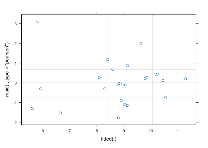

Figure 12.1: Graphical analyses of residuals for a split-plot ANOVA model

After having made sure that the basic assumptions for linear models hold, we can proceed to variance partitioning. In this case, we use the anova() method for a mixed model object, which gives a slightly different output than the anova() method for a linear model object. As the second argument, it is necessary to indicate the method we want to use to estimate the degrees of freedom, which, in mixed models, are not as easy to calculate as in linear models.

anova(mod.split, ddf="Kenward-Roger")
## Type III Analysis of Variance Table with Kenward-Roger's method
##                      Sum Sq Mean Sq NumDF DenDF F value
## Block                3.6596  1.2199     3     6  0.6521
## Tillage             23.6565 11.8282     2     6  6.3228
## WeedControl          3.3205  3.3205     1     9  1.7750
## Tillage:WeedControl 19.4641  9.7321     2     9  5.2023
##                      Pr(>F)  
## Block               0.61016  
## Tillage             0.03332 *
## WeedControl         0.21552  
## Tillage:WeedControl 0.03152 *
## ---
## Signif. codes:  
## 0 '***' 0.001 '**' 0.01 '*' 0.05 '.' 0.1 ' ' 1

From the above table we see that the ‘tillage by weed control method’ interaction is significant and, therefore, we show the means for the corresponding combinations of experimental factors. As in previous chapters, we use the emmeans() function.

library(emmeans)
meansAB <- emmeans(mod.split, ~Tillage:WeedControl)
multcomp::cld(meansAB, Letters = LETTERS)
##  Tillage WeedControl emmean    SE   df lower.CL upper.CL
##  MIN     PART          6.00 0.684 14.4     4.53     7.46
##  SP      PART          8.48 0.684 14.4     7.01     9.94
##  MIN     TOT           8.98 0.684 14.4     7.52    10.45
##  SP      TOT           9.14 0.684 14.4     7.68    10.60
##  DP      TOT           9.21 0.684 14.4     7.74    10.67
##  DP      PART         10.63 0.684 14.4     9.17    12.09
##  .group
##   A    
##   AB   
##   AB   
##   AB   
##    B   
##    B   
## 
## Results are averaged over the levels of: Block 
## Degrees-of-freedom method: kenward-roger 
## Confidence level used: 0.95 
## P value adjustment: tukey method for comparing a family of 6 estimates 
## significance level used: alpha = 0.05 
## NOTE: Compact letter displays are a misleading way to display comparisons
##       because they show NON-findings rather than findings.
##       Consider using 'pairs()', 'pwpp()', or 'pwpm()' instead.

We see that we should avoid controlling the weeds only along the crop rows, if we have not plowed the soil, at least to a shallow depth.

12.2 Example 2: a strip-plot design

In Chapter 2 we have also seen another possible arrangement of plots, relating to an experiment where three crops (sugarbeet, rape and soybean) were sown 40 days after an herbicide treatment. The aim was to assess possible phytotoxicity effects relating to an excessive persistence of herbicide residues in soil and the untreated control was added for the sake of comparison.

Figure 2.10 shows that each block was organised with three rows and two columns: the three crops were sown along the rows and the two herbicide treatments (rimsulfuron and the untreated control) were allocated along the columns. In this design, the observations are clustered in three groups:

the blocks
the rows within each block (three rows per block)
the columns within each block (two columns per block)

Analogously to the split-plot design, the rows represent the main plots for the crop factor, while the columns represent the main-plots for the herbicide factor. Both these grouping factors must be referenced as random effects in the model. The combinations between crops and herbicide treatments are allocated to the sub-plots, resulting from crossing the rows with the columns.

The dataset for this experiment, with four replicates, is available in the ‘recropS.csv’ file, that can be loaded from the usual repository. After loading, we transform all explanatory variables into factors. Furthermore, we create the definition of rows and columns, by considering that each row is uniquely defined by a specific block and crop and each column is uniquely defined by a specific herbicide and block.

rm(list=ls())
dataset <- read.csv("https://www.casaonofri.it/_datasets/recropS.csv")
head(dataset)
##     Herbicide     Crop Block CropBiomass
## 1       Check soyabean     1    199.0831
## 2       Check soyabean     2    257.3081
## 3       Check soyabean     3    345.5538
## 4       Check soyabean     4    210.8574
## 5 rimsulfuron soyabean     1    225.5651
## 6 rimsulfuron soyabean     2    195.3952
dataset$Herbicide <- factor(dataset$Herbicide)
dataset$Crop <- factor(dataset$Crop)
dataset$Block <- factor(dataset$Block)
dataset$Rows <- factor(dataset$Crop:dataset$Block)
dataset$Columns <- factor(dataset$Herbicide:dataset$Block)

12.2.1 Model definition

A good candidate model is:

\[Y_{ijk} = \mu + \gamma_k + \alpha_i + \theta_{ik} + \beta_j + \zeta_{jk} + \alpha\beta_{ij} + \varepsilon_{ijk}\]

where \(\mu\) is the intercept, \(\gamma_k\) are the block effects, \(\alpha_i\) are the crop effects \(\theta_ik\) are the random row effects, \(\beta_j\) are the herbicide effects, \(\zeta_{jk}\) are the random column effects, \(\alpha\beta_{ij}\) are the ‘crop by herbicide’ interaction effects and \(\varepsilon_ijk\) is the residual random error term. The three random effects are assumed as gaussian, with mean equal to zero and variances respectively equal to \(\sigma_{\theta}\), \(\sigma_{\zeta}\) and \(\sigma\).

12.2.2 Model fitting with R

At this stage, the code for model fitting should be straightforward, as well as that for variance partitioning

model.strip <- lmer(CropBiomass ~ Block + Herbicide*Crop + 
    (1|Rows) + (1|Columns), data = dataset)
anova(model.strip, ddf = "Kenward-Roger")
## Type III Analysis of Variance Table with Kenward-Roger's method
##                Sum Sq Mean Sq NumDF  DenDF F value  Pr(>F)
## Block           21451  7150.3     3 4.1367  2.5076 0.19387
## Herbicide         148   147.9     1 3.0000  0.0519 0.83450
## Crop            43874 21936.9     2 6.0000  7.6932 0.02208
## Herbicide:Crop  12549  6274.4     2 6.0000  2.2004 0.19198
##                 
## Block           
## Herbicide       
## Crop           *
## Herbicide:Crop  
## ---
## Signif. codes:  
## 0 '***' 0.001 '**' 0.01 '*' 0.05 '.' 0.1 ' ' 1

We see that only the crop effect is significant and, thus, we can be reasonably sure that the herbicide did not provoke unwanted carry-over effects to the crops sown in treated soil 40 days after the treatment.

12.3 Further readings

Bates, D., Mächler, M., Bolker, B., Walker, S., 2015. Fitting Linear Mixed-Effects Models Using lme4. Journal of Statistical Software 67. https://doi.org/10.18637/jss.v067.i01
Gałecki, A., Burzykowski, T., 2013. Linear mixed-effects models using R: a step-by-step approach. Springer, Berlin.
Kuznetsova, A., Brockhoff, P.B., Christensen, H.B., 2017. lmerTest Package: Tests in Linear Mixed Effects Models. Journal of Statistical Software 82, 1–26.