Chapter 6 Making Decisions under uncertainty
“… the null hypothesis is never proved or established, but it is possibly disproved, in the course of experimentation. Every experiment may be said to exist only to give the facts a chance of disproving the null hypothesis. (R. A. Fisher)
In Chapter 5 we have seen that experimental errors and, above all, sampling errors, produce uncertainty in the estimation process, which we have to account for by determining and displaying standard errors and confidence intervals. In the very same fashion, we need to be able to make decisions in presence of uncertainty; is the effect of a treatment statistically significant? Is the effect of a treatment higher/lower than the effect of another treatment?
Making such decisions is called Formal Hypothesis Testing (FHT) and we will see that this is mainly based on the so-called P-value. As usual, I will introduce the problem by using an example.
6.1 Comparing sample means: the Student’s t-test
6.1.1 The dataset
We have planned an experiment where we have compared the yield of genotype A with the yield of the genotype P and the experiment is laid down according to a completely randomised design with five replicates. This is a small-plot experiment with 10 plots, which need to be regarded as sampled from a wider population of plots; as we mentioned in the previous chapter, our interest is not in the sample, but it is in the population of plots, which means that we are looking for conclusions of general validity.
The results (in quintals per hectare) are the following:
As usual we calculate the descriptive statistics (mean and standard deviation) for each sample:
mA <- mean(A)
mP <- mean(P)
sA <- sd(A)
sP <- sd(P)
mA; sA
## [1] 70.2
## [1] 4.868265
mP; sP
## [1] 85.4
## [1] 5.727128
We see that the mean for the genotype P is higher than the mean for the genotype A, but such descriptive statistics are not sufficient to our aims. Therefore, we calculate standard errors, to express our uncertainty about the population means, as we have shown in the previous chapter.
Consequently, we can produce interval estimates for the population means, i.e., 85.4 \(\pm\) 5.12 and 70.2 \(\pm\) 4.35. We note that the confidence intervals do not overlap, which supports the idea that P is better than A, but we would like to reach a more formal decision.
First of all, we can see that the observed difference between \(m_A\) and \(m_P\) is equal to:
However, we are not interested in the above difference, but we are interested in the population difference, i.e. \(\mu_A - \mu_P\). We know that both the means have a certain degree of uncertainty, which propagates to the difference. In the previous chapter, we have seen that the variance of the sum/difference of independent samples is equal to the sum of variances; therefore, the standard error of the difference (SED) is equal to:
\[SED = \sqrt{ SEM_1^2 + SEM_2^2 }\]
In our example, the SED is:
It is intuitively clear that the difference (in quintals per hectare) should be regarded as significant when it is much higher than its standard error; indeed, this would mean that the difference is stronger than the uncertainty with which we have estimated it. We can formalise such an intuition by defining the \(T\) statistic for the sample difference:
\[T = \frac{m_A - m_P}{SED}\]
which is equal to:
If T is big, the difference is likely to be significant (not due to random effects); however, \(T\) is a sample statistic and it is expected to change whenever we repeat the experiment. How is the sampling distribution for \(T\)? To answer this question, we should distinguish two possible hypotheses about the data:
- Hypothesis 1. There is no difference between the two genotypes (null hypothesis: \(H_0\)) and, consequently, we have only one population and the two samples A and P are extracted from this population.
- Hypothesis 2. The two genotypes are different (alternative hypothesis: \(H_1\)) and, consequently, the two samples are extracted from two different populations, one for the A genotype and the other one for the P genotype.
In mathematical terms, the null hypothesis is:
\[H_0: \mu_1 = \mu_2 = \mu\]
The alternative hypothesis is:
\[H_1 :\mu_1 \neq \mu_2\]
More complex alternative hypotheses are also possible, such as \(H_1 :\mu _1 > \mu _2\), or \(H_1 :\mu _1 < \mu _2\). However, hypotheses should be set before looking at the data (according to the Galilean principle) and, in this case, we have no prior knowledge to justify the selection of one of such complex hypotheses. Therefore, we select the simple alternative hypothesis.
Which of the two hypotheses is more reasonable, by considering the observed data? We have seen that, according to the Popperian falsification principle, experiments should be planned to falsify hypotheses. Therefore, we take the null hypothesis and see whether we can falsify it.
This is one hint: if the null hypothesis were true, we should observe \(T = 0\), while we have observed \(T = -4.521727\). Is this enough to reject the null? Not at all, obviously. Indeed, the sample means can change from one experiment to the other and it is possible to obtain \(T \neq 0\) also when the experimental treatments are, indeed, the same treatment. Therefore, we need to ask ourselves: what is the sampling distribution for \(T\) under the null hypothesis?
6.1.2 Monte Carlo simulation
We can easily build an empirical sampling distribution for \(T\) by using Monte Carlo simulation. Look at the code in the box below: we use the for() statement to repeat the experiment 100,000 times. Each experiment consists of getting two samples of five individuals from the same population, with mean and standard deviation equal to the overall mean/standard deviation of the two original samples A and P. For each of the 100,000 couples of samples, we calculate T and store the result in the ‘result’ vector, which, in the end, represents the sampling distribution we were looking for.
# We assume a single population
mAP <- mean(c(A, P))
devStAP <- sd(c(A, P))

# we repeatedly sample from this common population
set.seed(34)
result <- rep(0, 100000)
for (i in 1:100000){
  sample1 <- rnorm(5, mAP, devStAP)
  sample2 <- rnorm(5, mAP, devStAP)
  SED <- sqrt( (sd(sample1)/sqrt(5))^2 +
                 (sd(sample2)/sqrt(5))^2 )
  result[i] <- (mean(sample1) - mean(sample2)) / SED
}
mean(result)
## [1] -0.001230418
min(result)
## [1] -9.993187
max(result)
## [1] 9.988315
What values did we obtain for \(T\)? On average, the values are close to 0, as we expected, considering that both samples were always obtained from the same population. However, we also note pretty high and low values (close to 10 and -10), which proves that random sampling fluctuations can also bring to very ‘odd’ results. For our real experiment we obtained \(T = -4.521727\), although the negative sign is just an artifact, relating to how we sorted the two means: we could have as well obtained \(T = 4.521727\).
Ronald Fisher proposed that we should reject the null, based on the probability of obtaining values as extreme or more extreme than those we observed, when the null is true. Looking at the vector ‘result’ we see that the proportion of values lower than -4.521727 and higher than 4.521727 is \(0.00095 + 0.00082 = 0.00177\). This is the so called P-value (see the code below).
length(result[result < Ti]) / 100000
## [1] 0.00095
length(result[result > - Ti]) /100000
## [1] 0.00082
Let’s summarise. We have seen that, when the null is true, the sampling distribution for \(T\) contains a very low proportion of values outside the interval from -4.521727 to 4.521727. Therefore, our observation fell in a very unlikely range, corresponding to a probability of 0.00177 (P-value = 0.00177); the usual yardstick for decision is 0.05, thus we reject the null. We do so, because, if the null were true, we would have obtained a very unlikely result; in other words, our scientific evidence against the null is strong enough to reject it.
6.1.3 A formal solution
A new question: is there any formal PDF, which we can use in place of our empirical, Monte-Carlo based sampling distribution for T? Let’s give a closer look at the ‘result’ vector. In particular, we can bin this continuous variable and plot the empirical distribution of frequencies (see Figure 6.1)
#Sampling distribution per T

b <- seq(-10, 10, by=0.25)
hist(result, breaks = b, freq=F,
  xlab = expression(paste(m)), ylab="Density",
  xlim=c(-10,10), ylim=c(0,0.45), main="")
curve(dnorm(x), add=TRUE, col="blue", n = 10001)
curve(dt(x, 8), add=TRUE, col="red", n = 10001)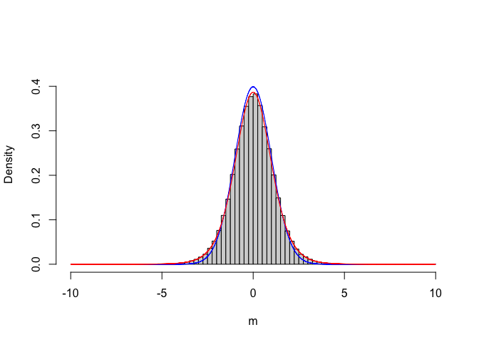
Figure 6.1: Empirical sampling distribution for the T statistic, compared to a standardised gaussian (blue line) and a Student’s t distribution with 8 degree of freedom (red line)
We see that the empirical distribution is not exactly standardised gaussian, but it can be described by using another type of distribution, that is the Student’s t distribution, with eight degrees of freedom (i.e. the sum of the degrees of freedom for the two samples). Now that we know this, instead of making a time consuming Monte Carlo simulation, we can use the Student’s t CDF to calculate the P-value, as shown in the box below.
pt(Ti, df=8) # probability that T > 4.5217
## [1] 0.0009727349
pt(-Ti, df=8, lower.tail = F) # probability that T < -4.5217
## [1] 0.0009727349
2 * pt(Ti, df=8) #P-value
## [1] 0.00194547
We see that the P-value is very close to that obtained by using simulation.
6.1.4 The t test with R
What we have just described is known as the Student’s t-test and it is often used to compare the means of two samples. The null hypothesis is that the two samples are drawn from the same populations and, therefore, their means are not significantly different. In practice, what we do is:
- Calculate the means and standard errors for the two samples
- Calculate the difference between the means
- Calculate the SED
- Calculate the observed \(T\) value
- Use the Student’s t CDF to retrieve the probabilities \(P(t < -T)\) and \(P(t > T)\)
- Reject the null hypothesis if the sum of the above probabilities is lower than 0.05.
More simply, we can reach the same solution by using the t.test() function in R, as shown in the box below.
t.test(A, P, paired = F, var.equal = T)
##
##  Two Sample t-test
##
## data:  A and P
## t = -4.5217, df = 8, p-value = 0.001945
## alternative hypothesis: true difference in means is not equal to 0
## 95 percent confidence interval:
##  -22.951742  -7.448258
## sample estimates:
## mean of x mean of y
##      70.2      85.4
Perhaps, it is worth to discuss the meaning of the two arguments ‘paired’ and ‘var.equal’, which were set, respectively, to FALSE and TRUE. In some cases two measures are taken on the same subject and we are interested in knowing whether there is a significant difference between the first and the second measure. For example, let’s imagine that we have given a group of five cows a certain drug and we have measured some blood parameter before and after the treatment. We would have a dataset composed by ten values, but we would only have five subjects, which would make a big difference with respect to our previous example.
In such a condition we talk about a paired t-test, which is performed by setting the argument ‘paired’ to TRUE, as shown in the box below.
t.test(A, P, paired = T, var.equal = T)
##
##  Paired t-test
##
## data:  A and P
## t = -22.915, df = 4, p-value = 2.149e-05
## alternative hypothesis: true mean difference is not equal to 0
## 95 percent confidence interval:
##  -17.04169 -13.35831
## sample estimates:
## mean difference
##           -15.2
The calculations are totally different and, therefore, the significance is, as well, different. In particular, we consider the five pairwise differences, their mean and their standard error, as shown below:
One further difference is that, as we have five subjects instead of ten, we only have four degrees of freedom.
In relation to the argument ‘var.equal’, you have perhaps noted that we made our Monte Carlo simulation by drawing samples from one gaussian distribution. However, the two samples might come from two gaussian distributions with the same mean and different standard deviations, which would modify our sampling distribution for \(T\), so that our P-level would become invalid. We talk about heteroscedasticity when the populations, and therefore the two samples, have different standard deviations. Otherwise we talk about homoscedasticity.
If we have reasons to suppose that the two samples come from populations with different standard deviations, we should use a heteroscedastic t-test (better known as Welch test). We can set the ‘var.equal’ argument to FALSE, as shown in the box below.
t.test(A, P, paired = F, var.equal = F)
##
##  Welch Two Sample t-test
##
## data:  A and P
## t = -4.5217, df = 7.7977, p-value = 0.002076
## alternative hypothesis: true difference in means is not equal to 0
## 95 percent confidence interval:
##  -22.986884  -7.413116
## sample estimates:
## mean of x mean of y
##      70.2      85.4
We see that the test is slightly less powerful (lower P-value), due to a reduced number of degrees of freedom, that is approximated by using the Satterthwaite formula:
\[DF_s \simeq \frac{ \left( s^2_1 + s^2_2 \right)^2 }{ \frac{(s^2_1)^2}{DF_1} + \frac{(s^2_2)^2}{DF_2} }\]
which reduces to:
\[DF_s = 2 \times DF\]
when the two samples are homoscedastic (\(s_1 = s_2\)).
in our example:
How do we decide whether the two samples have the same standard deviation and thus we can use a homoscedastic t-test? In general, we use a heteroscedastic t-test whenever the standard deviation for one sample is twice or three times as much with respect to the other, although some statisticians suggest that we should better use a heteroscedastic t-test in all cases, in order to increase our protection level against wrong rejections.
6.2 Comparing proportions: the \(\chi^2\) test
The t-test is very useful, but we can only use it with quantitative variables. What if we have a nominal response, e.g. death/alive, germinated/ungerminated? Let’s imagine an experiment where we have sprayed two populations of insects with an insecticide, respectively with or without an adjuvant. From one population (with adjuvant), we get a random sample of 75 insects and record 56 deaths, while from the other population (without adjuvant) we get a random sample of 50 insects and record 48 deaths.
In this case the sample efficacies are \(p_1 = 56/75 = 0.747\) and \(p_2 = 0.96\), but we are not interested in the samples, but in the whole populations, from where we sampled our insects.
If we remember Chapter 3, we may recall that the results of such an experiment reduce to a contingency table, as shown in the box below:
counts <- c(56, 19, 48, 2)
tab <- matrix(counts, 2, 2, byrow = T)
row.names(tab) <- c("I", "IA")
colnames(tab) <- c("D", "A")
tab <- as.table(tab)
tab
##     D  A
## I  56 19
## IA 48  2
For such a table, we already know how to calculate a \(\chi^2\), which measures the dependency among the two traits (insecticide treatment and deaths); the observed value, for our sample, is 9.768 (see below).
summary(tab)
## Number of cases in table: 125
## Number of factors: 2
## Test for independence of all factors:
##  Chisq = 9.768, df = 1, p-value = 0.001776
Clearly, like any other sample based statistic, the value of \(\chi^2\) changes any time we repeat the sampling effort. Therefore, the null hypothesis is:
\[H_o :\pi_1 = \pi_2 = \pi\]
Please, note that we make a reference to the populations, not to the samples. If this is true, what is the sampling distribution for \(\chi^2\)? And, what is the probability of obtaining a value of 9.768, or higher?
Although it is possible to set up a Monte Carlo simulation to derive an empirical distribution, we will not do so, for the sake of brevity. We anticipate that the sampling distribution for \(\chi^2\) can be described by using the \(\chi^2\) density function, with the appropriate number of degrees of freedom (the minimum between the number of columns and the number of rows, minus 1). In our case, we have only one degree of freedom and we can use the cumulative \(\chi^2\) distribution function to derive the probability of obtaining a value of 9.768, or higher:
The P-value is much lower than 0.05 and thus we can reject the null. We can get to the same result by using the chisq.test() function:
chisq.test(tab, correct = F)
##
##  Pearson's Chi-squared test
##
## data:  tab
## X-squared = 9.768, df = 1, p-value = 0.001776
Please, note the argument ‘correct = F’. A chi-square test is appropriate only when the number of subjects is high enough, e.g. higher than 30 subjects, or so. If not, we should improve our result by applying the so-called continuity correction, by using the argument ‘correct = T’, that is the default option in R.
6.3 Correct interpretation of the P-value
We use the P-value as the tool to decide whether we should accept or reject the null, i.e. we use it as an heuristic tool, which was exactly Ronald Fisher’s original intention. Later work by Jarzy Neyman and Egon Pearson, around 1930, gave the P-value a slightly different meaning, i.e. the probability of wrongly rejecting the null (so-called type I error rate: false positive). However, we should interpret such a probability with reference to the sampling distribution, not with reference to a single experiment. It means that we can say that: if the null is true and we repeat the experiment an infinite number of times, we have less than 5% probability of obtaining such a high T or \(\chi^2\) value. On the other hand, we cannot legitimately conclude our experiment by saying that: there is less then 5% probability that we have reached wrong conclusions. Indeed, we do not (and will never) know whether we have reached correct conclusions in our specific experiment, while our ‘false-positive’ probability is only valid on the long run.
6.4 Conclusions
The intrinsic uncertainty in all experimental data does not allow us to reach conclusions and make decisions with no risk of error. As our aim is to reject hypotheses, we protect ourself as much as possible against the possibility of wrong rejection. To this aim, we use the P-value for the null hypothesis: if this is lower than the predefined yardstick level (usually \(\alpha = 0.05\)) we reject the null and we can be confident that such an heuristic, in the long run, will result in less than 5% of wrong rejections.
Before concluding, we should point out that we do not only run the risk of committing a false-positive error (type I error), we also run the risk of committing a false negative error (type II error), whenever we fail to reject a false null hypothesis. These two type of errors are nicely put in Figure 6.2, that is commonly available in the web.
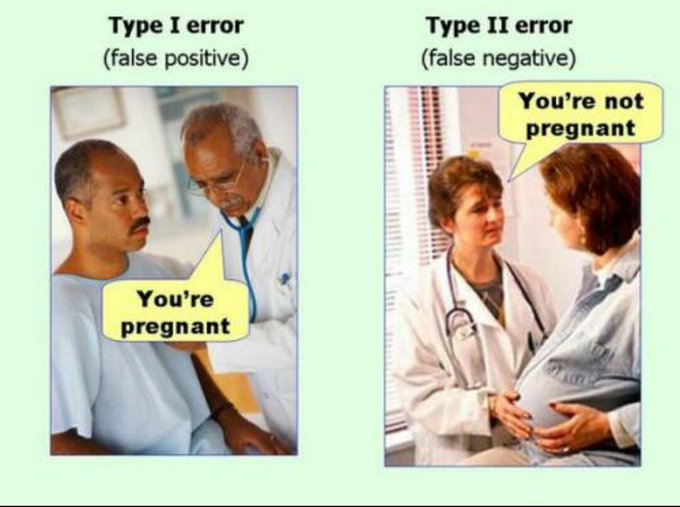
Figure 6.2: The two types of statistical errors
Please, also note that the two error types are interrelated and the highest the protection against the false-positive error, the highest the risk of committing a false negative error. In general, we should be always careful to decide which of the two errors might be more dangerous for our specific aim.