A motivating examples

In recent times, we wanted to model the effect of temperature on seed germination for Hordeum vulgare and we made an assay with three replicated Petri dishes (50 seeds each) at 9 constant temperature levels (1, 3, 7, 10, 15, 20, 25, 30, 35, 40 °C). Germinated seeds were counted and removed daily for 10 days. This unpublished dataset is available as barley in the drcSeedGerm package, which needs to be installed from github (see below), together with the drcte package for time-to-event model fitting. The following code loads the necessary packages, loads the datasets and shows the first six lines.

# Installing packages (only at first instance)
# library(devtools)
# install_github("OnofriAndreaPG/drcSeedGerm")
# install_github("OnofriAndreaPG/drcte")
library(drcSeedGerm)
library(tidyverse)
data(barley)
head(barley)
##   Dish Temp timeBef timeAf nSeeds nCum propCum
## 1    1    1       0      1      0    0       0
## 2    1    1       1      2      0    0       0
## 3    1    1       2      3      0    0       0
## 4    1    1       3      4      0    0       0
## 5    1    1       4      5      0    0       0
## 6    1    1       5      6      0    0       0

In this dataset, ‘timeAf’ represents the moment when germinated seeds were counted, while ’timeBef’ represents the previous inspection time (or the beginning of the assay). The column ’nSeeds’ is the number of seeds that germinated during each time interval between ‘timeBef’ and ‘timeAf. For the analyses, we will also make use of the ’Temp’ (temperature) and ‘Dish’ (Petri dish) columns.

This dataset was already analysed in Onofri et al. (2018; Example 3 and 4) by using the same methodology, but a different R coding (see the Supplemental Material in that paper), that is now outdated. This post will show you the updated coding.

A first thermal-time model

As we have shown in previous posts (see here and here), the effect of environmental covariates (temperature, in this case) can be simply included by independently coding a different time-to-event curve to each level of that covariate. In other words, considering that a parametric time-to-event curve is defined as a cumulative probability function (\(\Phi\)), with three parameters:

\[P(t) = \Phi \left( b, d, e \right)\] where \(P(t)\) is the cumulative probability of germination at time \(t\), \(e\) is the median germination time, \(b\) is the slope at the inflection point and \(d\) is the maximum germinated proportion, the most obvious extension is to allow for different \(b\), \(d\) and \(e\) values for each of the i^th temperature levels (\(T\)):

\[P(t, T) = \Phi \left( b_i, d_i, e_i \right)\] Although the above approach is possible, we will not purse it here, as it is clearly sub-optimal; indeed, such an approach wrongly considers the temperature as a factor, i.e. a set of nominal classes with no intrinsic orderings and distances. Obviosly, we should better regard the temperature as a continuous variable, by coding a time-to-event model where the three parameters are expressed as continuous functions of \(T\):

\[P(t, T) = \Phi \left[ b(T), d(T), e(T) \right]\]

For the ‘phalaris’ dataset (Onofri et al., 2018; example 3) we used a log-logistic cumulative distribution function, with the following sub-models:

\[ \left\{ {\begin{array}{{l}} P(t, T) = \frac{ d(T) }{1 + \exp \left\{ b \left[ \log(t) - \log( e(T) ) \right] \right\} } \\ d(T) = G \, \left[ 1 - \exp \left( - \frac{ T_c - T }{\sigma_{T_c}} \right) \right] \\ 1/[e(T)] = GR_{50}(T) = \frac{T - T_b }{\theta_T} \left[1 - \frac{T - T_b}{T_c - T_b}\right] \\ \end{array}} \right. \quad \quad (\textrm{TTEM})\]

Please, note that the shape parameter \(b\) has been regarded as independent from temperature; the parameters are:

1. \(G\), that is the germinable fraction, accounting for the fact that \(d\) may not reach 1, regardless of time and temperature;
2. \(T_c\), that is the ceiling temperature for germination;
3. \(\sigma_{T_c}\), that represents the variability of \(T_c\) within the seed lot;
4. \(T_b\), that is the base temperature for germination;
5. \(\theta_T\), that is the thermal-time parameter;
6. \(b\), that is the scale parameters for the log-logistic distribution.

You can get more information from our original paper (Onofri et al., 2018). This thermal-time model was implemented in R as the TTEM() function, and it is available within the drcSeedGerm package; we can fit it by using the drmte() function in the drcte package, with no need to provide starting values for model parameters, because a self-starting routine is available. The summary() method can be used to retrieve the parameter estimates.

# Thermal-Time-to-event model fit
modTTEM <- drmte( nSeeds ~ timeBef + timeAf + Temp, data=barley,
               fct=TTEM())
summary(modTTEM, units = Dish)
## 
## Model fitted: Thermal-time model with shifted exponential for Pmax and Mesgaran model for GR50
## 
## Robust estimation: Cluster robust sandwich SEs 
## 
## Parameter estimates:
## 
##                       Estimate Std. Error t value  Pr(>|t|)    
## G:(Intercept)         12.46391    2.40502  5.1825 2.772e-07 ***
## Tc:(Intercept)        82.66899   23.47042  3.5223  0.000452 ***
## sigmaTc:(Intercept) 1018.92708  322.67791  3.1577  0.001649 ** 
## Tb:(Intercept)        -1.89327    0.38741 -4.8870 1.236e-06 ***
## ThetaT:(Intercept)    43.41025    4.37185  9.9295 < 2.2e-16 ***
## b:(Intercept)          5.62759    0.69149  8.1383 1.520e-15 ***
## ---
## Signif. codes:  0 '***' 0.001 '**' 0.01 '*' 0.05 '.' 0.1 ' ' 1

It is always important not to neglect a graphical inspection of model fit. The plot() method does not work with time-to-event curves with additional covariates (apart from time). However, we can retrieve the fitted data by using the plotData() function and use those predictions within the ggplot() function. The box below shows the appropriate coding; the red circles in the graphs represent the observed means, while the black lines are model predictions).

tab <- plotData(modTTEM)

ggplot() +
  geom_point(data = tab$plotPoints, mapping = aes(x = timeAf, y = CDF),
            col = "red") +
  geom_line(data = tab$plotFits, mapping = aes(x = timeAf, y = CDF)) +
  facet_wrap( ~ Temp) +
  scale_x_continuous(name = "Time (d)") +
  scale_y_continuous(name = "Cumulative proportion of germinated seeds")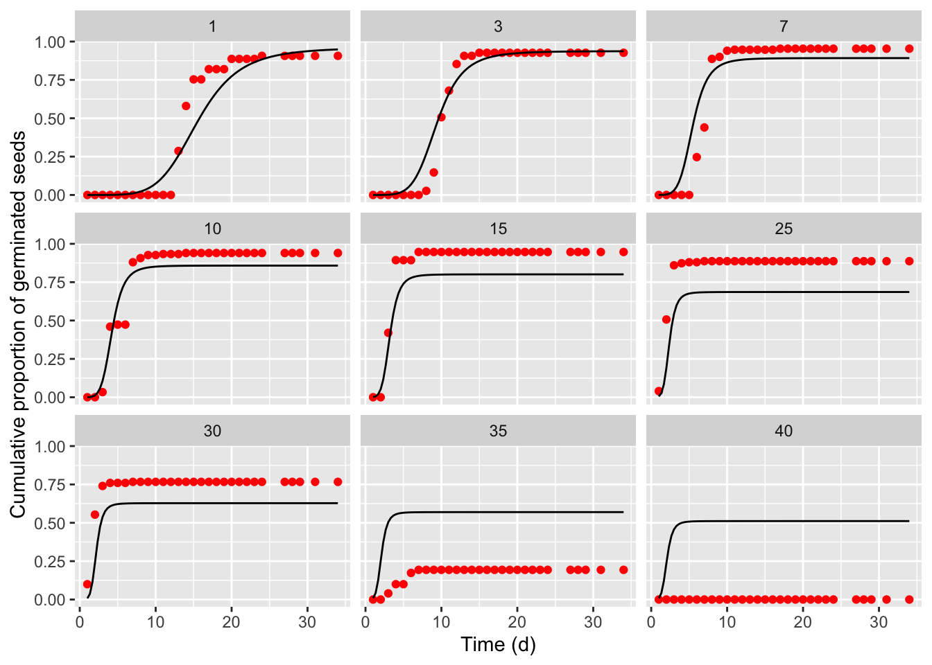

The previous graph shows that the TTEM() model, that we had successfully used with other datasets, failed to provide an adequate description of the germination time-course for barley. Therefore, we modified one of the sub-models, by adopting the approach highlighted in Rowse and Finch-Savage (2003), where:

\[1/[e(T)] = GR_{50}(T) = \left\{ {\begin{array}{ll} \frac{T - T_b}{\theta_T} & \textrm{if} \,\,\, T_b < T < T_d \\ \frac{T - T_b}{\theta_T} \left[ 1 - \frac{T - T_d}{T_c - T_d} \right] & \textrm{if} \,\,\, T_d < T < T_c \\ 0 & \textrm{if} \,\,\, T \leq T_b \,\,\, or \,\,\, T \geq T_c \end{array}} \right. \]

Furthermore, we also made a further improvement, by coding another model where also the \(b\) parameter was allowed to change with temperature, according to the following equation:

\[ \sigma(T) = \frac{1}{b(T)} = \frac{1}{b_0} + s (T - T_b)\]

These two improved models were coded as the TTERF() function (with the only change in the ‘e’ submodel), and as the TTERFc() function (with a change in both the ‘b’ and ‘e’ submodels), which are available within the drcSeedGerm package. The code below is used to fit both models and explore the resulting fits: the symbols show the observed means, the blue line represents the ‘TTERF’ fit and the red line represents the ‘TTERFc’ fit.

modTTERF <- drmte( nSeeds ~ timeBef + timeAf + Temp, data=barley,
               fct=TTERF())
modTTERFc <- drmte(nSeeds ~ timeBef + timeAf + Temp, data=barley,
               fct=TTERFc())
AIC(modTTEM, modTTERF, modTTERFc)
##            df      AIC
## modTTEM   804 6478.917
## modTTERF  803 5730.622
## modTTERFc 802 5602.532
tab2 <- plotData(modTTERF)
tab3 <- plotData(modTTERFc)

ggplot() +
  geom_point(data = tab$plotPoints, mapping = aes(x = timeAf, y = CDF),
            col = "red") +
  geom_line(data = tab2$plotFits, mapping = aes(x = timeAf, y = CDF),
            col = "blue") +
  geom_line(data = tab3$plotFits, mapping = aes(x = timeAf, y = CDF),
            col = "red") +
  facet_wrap( ~ Temp) +
  scale_x_continuous(name = "Time (d)") +
  scale_y_continuous(name = "Cumulative proportion of germinated seeds")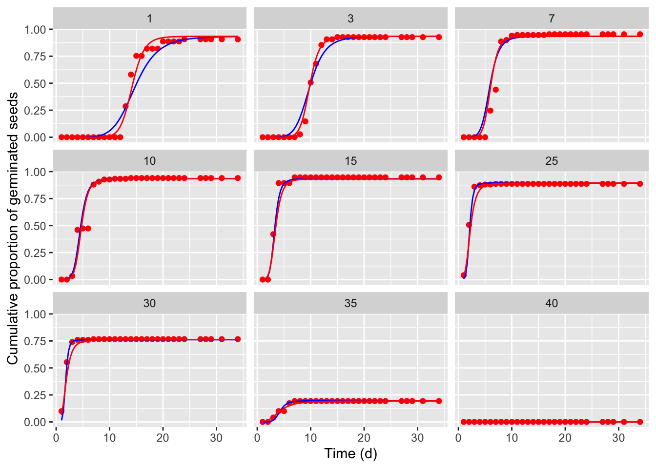

We see that, with respect to the TTEM model, both the two improved models provide a better fit.

It should be clear that this modelling approach is rather flexible, by appropriately changing one or more submodels, and it can fit the germination pattern of several species in several environmental conditions.

Thank you for reading!

Prof. Andrea Onofri
Department of Agricultural, Food and Environmental Sciences
University of Perugia (Italy)
Send comments to: andrea.onofri@unipg.it

References

1. Onofri, A., Benincasa, P., Mesgaran, M.B., Ritz, C., 2018. Hydrothermal-time-to-event models for seed germination. European Journal of Agronomy 101, 129–139.
2. Rowse, H.R., Finch-Savage, W.E., 2003. Hydrothermal threshold models can describe the germination response of carrot (Daucus carota) and onion (Allium cepa) seed populations across both sub- and supra-optimal temperatures. New Phytologist 158, 101–108.